Deep neural networks(DNNs) have become one of the most widely used algorithms in image classification (Krizhevsky et al., 2012), object detection (Ren et al., 2015), video analysis (Graves et al., 2013), and other fields with far surpassing accuracy than traditional algorithms. However, the high computing power and memory requirements of DNNs make it difficult for edge devices to deploy them with low latency, low power consumption, and high precision (Uddin and Nilsson, 2020; Veeramanikandan et al., 2020; Zhang et al., 2020; Fortino et al., 2021). To address this problem, various methods have been proposed for network compression and inference acceleration, including lightweight architecture design (Howard et al., 2017; Zhang X. et al., 2018), network pruning (LeCun et al., 1990; Hassibi and Stork, 1993; Li et al., 2016), weight quantization (Courbariaux et al., 2015; Hubara et al., 2017), matrix factorization (Denton et al., 2014), and knowledge distillation (Hinton et al., 2015; Gou et al., 2021). Quantization compresses the model by reducing the size of the weights or activations. Matrix factorization is to approximate the large number of redundant filters of a layer using a linear combination of fewer filters. And knowledge distillation trains another simple network by using the output of a pre-trained complex network as a supervisory signal. Among them, network pruning compresses the existing network to reduce the requirements for space and computing power, to achieve real-time operation on portable devices. According to the granularity of pruning, network pruning methods can be divided into structured and unstructured pruning. Unstructured pruning requires specialized hardware and software for effective reasoning, and random connections will lead to poor cache locality and memory jump access, which makes acceleration very limited. Among structured pruning methods, filter pruning has received widespread attention because of its advantages of being directly compatible with current general-purpose hardware and highly efficient basic linear algebra subprogram (BLAS) libraries. The research in this paper belongs to the category of structured pruning, that is, the pruning granularity is at the level of convolution kernels.

Formally, for a CNN with weights of W and L convolutional layers, and Ni filters in each layer, determining which filter needs to be pruned is a combinatorial optimization problem, that can be expressed as follows (Zhou et al., 2019):

h(F(l,nl))*W(nl,nl+1)    (2)

where W(nl,nl+1)∈ℝK×K is the nl-dimensional weight of the nl+1-th convolution kernel, corresponding to the nl+1-th input feature map. We explore and analyze the loss of representational power brought about by removing one of two similar feature channels and its filter. Suppose that F(l,i) and F(l,j) are two similar channels, deleting the F(l,i), then for the pruned Fp(l+1,nl+1) we have:

Fp(l+1,nl+1)=h(F(l,j))*(W(i,nl+1)+W(j,nl+1))     +∑nl≠i,jh(F(l,nl))*W(nl,nl+1)    (3)

We use mean squared error (MSE) to quantify the loss of the two feature maps before and after pruning:

L(F(l+1,nl+1),Fp(l+1,nl+1))=(Hl+1×Wl+1×B)-1×‖F(l+1,nl+1)-Fp(l+1,nl+1)‖22=1al+1‖(h(F(l,i))-h(F(l,j)))*W(i,nl+1)‖22    (4)

where al+1 = Hl+1×Wl+1×B. For each feature map Fp(l+1,nl+1) in the l+1-th convolutional layer, the loss caused by removing the feature map F(l,i) from the l-th convolutional layer, as defined in Equation (4), admits the following upper bound:

L(F(l+1,nl+1),Fp(l+1,nl+1))≤ε×minj∈L(F(l,i),F(l,j))    (5)

where ε=alal+1K2‖W(i,nl+1)‖22 and K2 corresponds to the size of each filter W(nl,nl+1). Detailed derivation can be found in Appendix. We can conclude from Equation (5) that E is determined by the size of the feature maps, the L2-norm of the convolution kernel and its weights. In experiments, E is usually a value of the order of 10−2, which means that the loss of removing one of the similar channels is negligible, as long as there are sufficiently similar channels to replace it.

In practice, our goal is to find similar channels and remove one of them. However, computing the similarity of channels directly has two apparent limitations. First, the activations of feature maps are affected differently by different batches of data. Second, calculating the similarity between all channels is inefficient for current large CNN architectures. To solve these issues, we use the convolution kernel as a unit for comparison. It can be seen from Equation (2) that when the input feature maps are the same, the feature maps obtained by similar convolution kernels are also identical, and the parameters of the kernels are not affected by the data batch. Intuitively, we quantify the similarity of two kernels by Euclidean distance, which is more commonly used in the analyses that need to reflect a difference in dimensions. In addition, Euclidean distance measures the distance between points in multidimensional space and can remember the absolute difference of characteristics. Therefore, for the lth convolutional layer:

D(l)=dist(Fl,j,Fl,k),0≤j≤Nl+1,j≤k≤Nl+1      =    (6)

where

dj,k=∑n=1Nl∑k1K∑k2=1K|Wj(n,k1,k2)-Wk(n,k1,k2)|2    (7)

Wj(n,k1,k2) is each weight in the filter F(l, j). For the lth convolution layer, we obtain a set of distances D(l), which contains the distances between the jth filter and all other filters. The smaller the distance is, the more significant the similarity between the two filters, indicating that the filter has extracted features similar to those of other filters.

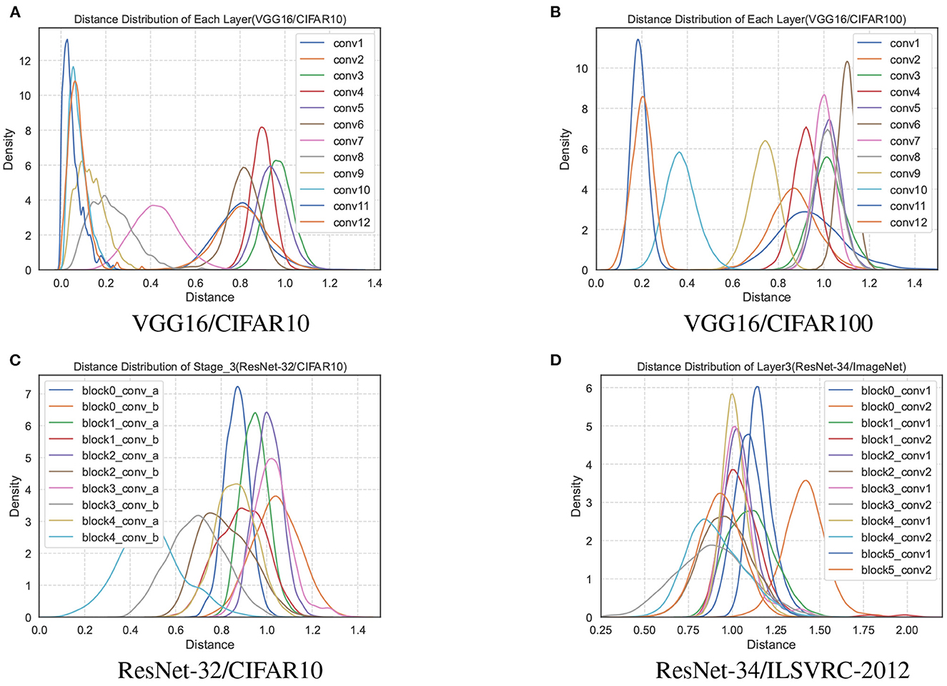
We remove the repeated distance with the same subscript in D(l), and perform statistical analysis on all values in the set. Statistics show an interesting phenomenon that the distance distribution of each layer is an approximately Gaussian distribution in the trained network, as shown in Figure 2. The distance sets D(l) of different layers in the network are distributed differently, and the mean value even differs by an order of magnitude. However, the distance distribution between the filters has partial jitters since the convolutional layers, such as conv1 and conv2 of the VGG16, are affected by the input data.

Figure 2. The distance distributions of each layer of the network model parameters trained by VGG16 on the CIFAR10 and CIFAR100 datasets are shown in (A, B). (C) The distance distribution of all convolutional layers in the third stage of ResNet-32/CIFAR10. (D) The third layer of ResNet-34/ILSVRC-2012.

3.2. Filter pruning based on similarity

After the distance distribution of each convolutional layer is obtained, how great can the distance between the two filters be determined to be similar? One of the methods is to get a minimum distance value min[D(l)] each time, that is, to remove one filter each time until the set requirement is reached. That is inefficient and laborious for network structures with thousands of convolution kernels. To obtain a set of redundant filters simultaneously, we first need to set a threshold λ, and a pair of filters corresponding to a distance less than this threshold are judged to be similar. Since the distance distribution of each convolutional layer is different, simply specifying the threshold of each layer will bring more hyperparameter problems. How can a reasonable threshold be set for each layer more efficiently with fewer hyperparameters?

Inspired by the empirical rule (3σ) of a Gaussian distribution, the probability of falling within [μ−σ, μ+σ] is 0.68:

P(i)(μ-σ≤x≤μ+σ)=0.68,x∈D(l)    (8)

we set a scaling factor α such that λ = μ − ασ ∈ (−∞, μ], and then α ∈ [0, +∞),

P(l)(dj,k(l)≤λ)=12πσ∫−∞λexp(−(x−μ)22σ2)dx                            t=x−μσ__12π∫−∞λ−μσexp(−t22)dt                          =12π∫−∞−αexp(−t22)dt                          =Φ(−α)=1−Φ(α)    (9)

where Φ(•) is the distribution function of the standard normal distribution, it can be obtained from checking the Standard normal distribution table: when α = 0, λ = μ, P = 0.5; and α → +∞, λ → −∞, P → 0. If dj,k(l)<μ-α*σ, the filters corresponding to dj,k(l) in the shaded part of Figure 1 are judged to be similar, and then dj,k(l) is selected as the candidate set Dselect(l):

dj,k(l)∈Dselect(l)j,k∈Fselect(l)    (10)

Fselect(l) is the set of indexes of the corresponding filters in Dselect(l). We use a hyperparameter α to get equal-probability candidate sets in different layers for different distance distributions in each layer.

It can be seen in the experiment that a filter satisfies similar conditions simultaneously with multiple filters, but how can we determine the final deleted filters in the candidate set. For the lth layer, we count the number of times of the jth appears in Fselect(l), denoted by Cj(l). Under extreme circumstances, if dj,k(l)<λ(0≤k≤Nl+1-1,k≠j) holds for the distance between the jth filter and all other filters, then Cj(l)=Nl+1-1. We use the proportional factor r ∈ [0, 1] to represent the frequency of the jth filter,

r=Cj(l)Nl+1-1    (11)

If Cj(l)>r*(Nl+1-1), then j∈Fpruned(l), Fpruned(l) is the set of final pruning filters. The above algorithm obtains a set of redundant filters for one convolution layer in the network structure, and the schematic diagram of the pruning process of each layer is shown in Figure 1.

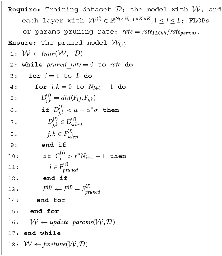
3.3. Compression recipes

In addition to the judgment method of network parameter redundancy, the pruning strategy, implementation and network structure are also essential factors that affect the compression performance. As the pruning rate increases, network performance loss increases, and the redundant judgment of parameters is also prone to deviation when the network parameters deviate from the optimal point. Previous work uses layer-by-layer pruning and fine-tuning strategies or retraining to reduce the judgment error caused by performance loss and iterates this process until the target compression rate is achieved. However, when the iteration parameter setting is small and the target compression rate is significant, the pruning period will greatly increase, and the training time cost will be very high. Therefore, we prune all layers at once instead of layer-by-layer pruning and fine-tuning, significantly reducing the pruning cost. After complete pruning, the computation and parameter quantity of the whole network are calculated. If the set pruning requirements are met, the pruning is completed; otherwise, the redundant filters will continue to be searched for further pruning on the network structure of the last pruning until the set pruning requirements are met (computational cost reduction or parameter reduction), as shown in Algorithm 1.

Algorithm 1. Iterative pruning algorithm.

In the implementation of pruning, He et al. (2018a) proposed not to directly delete the pruned parameters in the pruning process, which increases the fault tolerance of judgment. Many current works are based on soft pruning implementations, and for a fair comparison, we propose an iteration pruning strategy based on soft pruning. In the experiment, it is found that although the filters set to zero in the previous iteration are not deleted, they will not change in the subsequent fine-tuning no matter how the network is updated, which affects the distance calculation and redundant judgment. To solve this problem, we set a mask for each filter, the pruned filters are 0, and the others are 1, and the mask is updated by the algorithm in real-time in each iteration. When calculating the distance between the filters in one layer, the distance will be multiplied by the mask value corresponding to the two filters at the same time,

dj,k(l)=dist(Fl,j,Fl,k)*maskj*maskk=p2∈(δi,j(l)(p1,p2)*W(i,nl+1))2=1al+1∑p1∈p2∈|〈δi,j(l)(p1,p2),W(i,nl+1)〉|2    (16)

Applying Cauchy-Schwarz inequality, then:

ℒ(ℱ(l+1,nl+1),ℱp(l+1,nl+1))≤