1. Introduction

Electroencephalography (EEG) is a non-invasive method for recording and analyzing brain activity. Given the low amplitude of the recorded signal, even an eye blink or unintentional muscle contractions create noise in the recordings, complicating the identification of a patient's mental condition. To overcome this problem, researchers traditionally focused on handcrafted feature extraction based on e.g., short-time Fourier transform (STFT) (Griffin and Lim, 1984), discrete wavelet transform (DWT) (Shensa, 1992), or tensor decomposition (Naskovska et al., 2020) to remove noise and focus on the relevant signals. Typically, the generated spectrograms are represented as images and then classified by, e.g., feed-forward networks (FFNs) (Montana and Davis, 1989). Automation of such analyses not only requires high accuracy but their embedding into usage scenarios, such as neurofeedback applications (Hammond, 2007) or brain-computer interfaces (BCI) (Schalk et al., 2004) to classify mental states also require efficient processing. However, these methods have to be calibrated manually for the image generation when specific parameters, e.g., the sampling frequency, have changed. This step requires extensive expert knowledge as otherwise important features might be neglected during preprocessing. Furthermore, these methods can be time-consuming, if the number of EEG channels increases since some of the methods propose a window and channel-wise time-frequency analysis (Tabar and Halici, 2016). Hence, previous studies often merely evaluate their methods on low channel EEG data, i.e., fewer than the clinical routine of 21 channels (Tabar and Halici, 2016; Ni et al., 2017; Mert and Celik, 2021; Yilmaz and Kose, 2021).

In the last decade, gated recurrent neural networks (RNN) like long short term memory (LSTM) (Hochreiter and Schmidhuber, 1997) and gated recurrent unit (GRU) (Chung et al., 2014) have been demonstrated to yield superior results when analyzing and classifying time series without the need for complex preprocessing and hand-crafted feature extraction. Thereby, manual configuration effort and the need for expert knowledge in signal analysis can be drastically reduced, while achieving state of the art results. In order to increase the predictive power of these approaches, they face a constant evolution with notable improvements. Such improvements include bidirectional RNN topologies and the attention mechanism that has stimulated many new network topologies beyond RNNs. More recent studies, propose time-convolving neural networks and demonstrate that they can yield high predictive performance on time series like audio signals (Oord et al., 2016; Bai et al., 2018). More specifically, Bai et al. (2018) propose a network topology based on temporal convolutions, which achieves remarkable results on popular datasets thereby outperforming LSTM and GRU topologies. In contrast to these more complex approaches, also methods based on simplified RNNs like echo state networks (ESN) achieved good (Bozhkov et al., 2016), respectively even superior results (Sun et al., 2019). As a FFN based counterpart of ESNs we reference to extreme learning machines (ELM), which were utilized for EEG classification tasks by Tan et al. (2016) and Liang et al. (2006), reaching superior results while further reducing the computational complexity.

In this paper, we systematically compare a large variety of RNN and FFN topologies as well as the influence of topological variants, e.g., bidirectional networks and attention mechanisms for EEG analysis. We do not focus on a specific medical application, but rather aim to compare the performance of each network topology based on benchmark EEG recordings. To the best of our knowledge recurrent and feed-forward topologies have never been compared on the same EEG dataset and with the same preprocessing pipeline before. We evaluate all approaches on three different EEG datasets: the well-known benchmark DEAP, a seizure detection task, and an in-house frequency entrainment dataset. Thus, we aim to answer the following research questions:

(RQ 1)   Recurrent topologies: Which recurrent topology shows advantages for EEG time series classification in comparison between non-gated, gated, and random high dimensional mapping approaches?

(RQ 2)   Feed-Forward topologies: Are feed-forward topologies based on convolution and self-attention suitable for EEG time series classification without further preprocessing methods?

(RQ 3)   Advanced architectural concepts: Can extensions for LSTMs, like attention and bidirectionality, improve the performance for these networks for EEG time series classification?

Our results indicate that feed-forward networks yield advantages compared to RNNs without additional concepts. Nonetheless, applying attention to RNNs yielded notable performance increases and even surpasses feed-forward topologies for some of the investigated datasets.

The rest of the paper is organized as follows, Section 2 provides a brief summary of use cases and problems related to automated EEG analysis and introduces the step-by-step explanation of the typical workflow from the recording of the raw EEG signal to the final analysis result. Furthermore, the studied network topologies are discussed in detail. In addition, the different topological variations, like bidirectional networks and attention are explained. In this section, we will also explain the used datasets, input representation, and chosen parameters for each of the trained network architectures. In Section 3, we show different classification strategies and approaches mentioned by various publications based on the preprocessing methods and architectures used. Additionally, we discuss the different results for each of the presented topologies. Last, we discuss some limitations of our work, introduce potential future research directions and conclude on the different methods compared in this paper.

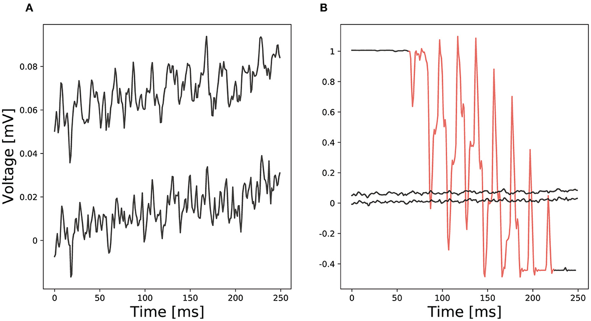
2. Methods 2.1. Applications and problems of EEG analysis

In general, analyzing EEG data is a challenging task with many difficulties (Vallabhaneni et al., 2021). Due to typically low amplitude signals in the μV range (cp. Figure 1A), small interferences can distort a signal making it unusable (cp. Figure 1B red section compared to ordinary EEG recordings). We denote an interference as any part of a signal that is not directly generated by brain activity or brain activity that is not directly produced as result of an experimental stimulus. It is hard to remove interferences from a signal since these often show similar characteristics as the actual signal. To remove transient interferences before analyzing an EEG signal, various methods have been proposed, e.g., linear regression or blind source separation (Urigüen and Garcia-Zapirain, 2015). Nevertheless, none of them is supposed to work perfectly and remaining interferences may cause erroneous analysis results (Hagmann et al., 2006).

Figure 1. Comparison of two EEG examples: (A) Ordinary EEG recordings from two different electrodes and (B) a red marked channel with transient interferences compared to ordinary EEG recordings.

Another problem can be the placement and number of electrodes that capture brain activity. Not all regions of the brain are equally active during experiments and some regions are more dominant than others. When less electrodes are used, activation could be missed during the recording which results in no features.

To avoid such errors it is advisable to use a higher number of electrodes and to cover all areas of the head. When the number of electrodes used increases, the time and effort required to preprocess the data increases as well. This can be critical for time-frequency transforms which typically process signals channel- or window-wise (Li et al., 2016; Tabar and Halici, 2016).

In recent years, deep learning neural network approaches have been applied to a wide range of neuroscientific problems like feedback on motor imagery tasks (MI) (Tabar and Halici, 2016), emotion recognition (Ng et al., 2015), seizure detection (Thodoroff et al., 2016) and many other tasks (Gong et al., 2021) (see Table 4). These studies typically apply standard convolutional and recurrent neural networks (Craik et al., 2019). Many studies use handcrafted features as input for deep neural networks. However, extracting features can be time-consuming and often requires expert domain knowledge to extract features which represent the signal correctly. To avoid loss of information during the preprocessing phase, the aim of neurobiological analysis should be an analysis of raw data. If more information is provided to the neural network, better results can be expected. To the best of our knowledge, no study exists that systematically compares feed-forward and recurrent neural networks in all their flavors for raw signal EEG data analysis.

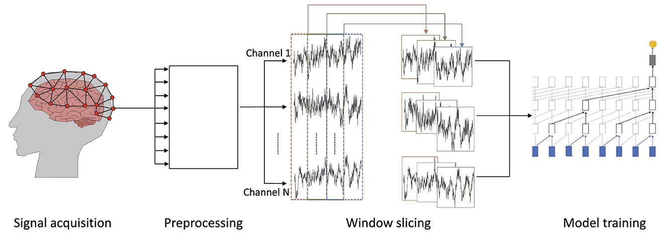
2.2. Automated EEG analysis workflow

In this subsection, we discuss the workflow for automated EEG data analysis from the recording of data to the eventual prediction (cp. Figure 2).

Figure 2. Overview of the workflow for processing EEG data: (1) signal acquisition—EEG data are recorded, (2) preprocessing—recorded data are preprocessed and noise is removed by filters, (3) window slicing—the resulting waveforms are divided into windows of equal size, which may overlap, and (4) model training—on the windowed and preprocessed wave forms.

2.2.1. Signal acquisition

We focus on EEG recordings as a non-invasive and cost efficient method to measure brain activity with electrodes placed directly on the scalp (Craik et al., 2019) (cp. Figure 2).

2.2.2. Preprocessing

Preprocessing of data, such as filtering the signal and removing interferences, is an important part of training neural networks in general. Poorly preprocessed data ultimately yield poor network inference performance which can hardly be compensated by training methodology and network topology (Hagmann et al., 2006). This processing is particularly important for EEG signals which, due to their low amplitude, can be strongly altered by only small influences such as unintended muscle contractions. For this reason, almost all EEG data are bandpass filtered directly after recording to remove noise distorting the signal. An often used frequency range for EEG data analysis is 1–40 Hz. The filter range might also depend on the experimental setup during the EEG recording. Transient interference removal is another important part of preprocessing. Interferences influence a signal in a significant way and often even distort a signal such that it is nearly impossible to recognize its actual waveform (cp. Figure 1). Different methods such as linear regression or blind source separation were proposed to remove interferences. For heavily distorted signals, like shown in Figure 1 a threshold detection can track and remove the interference. After removing interferences and noise, the preprocessed data can be used as input for deep neural networks.

2.2.3. Window slicing

EEG signals may contain many data points, depending on the sampling rate and duration of a recording. Often, it is not feasible to analyze a complete recording due to prohibitive compute and memory requirements which result from an excessive input length. It is, therefore, common to apply window slicing to generate data frames and to incrementally analyze these smaller snippets of a signal rather than a whole recording at once (Tabar and Halici, 2016; Gao et al., 2019). Thereby, the size of a window and a potential overlap of successive windows are hyper-parameters of the respective analysis and depend on its goal (cp. middle of Figure 2). For example, the detection of slow theta brain waves requires larger windows to capture a full wave within the window while alpha and beta brain waves can be captured in a smaller window.

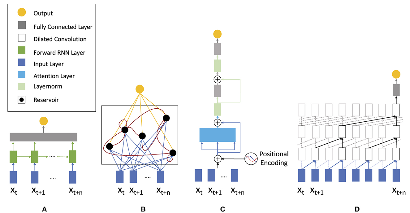
2.2.4. Model training

The goal here is to select, parameterize, and train a suitable model architecture. Below, we discuss model topologies applicable for analyzing and specifically classifying EEG time series data (cp. Figure 3), which we then systematically evaluate on different EEG datasets in Section 2.5. Once the initial architectural choice is made, hyper-parameters are varied and optimized to improve prediction performance results. In this work we study a variety of different topolgies. These include the basic RNN as well as the most prominent recurrent networks GRU and LSTM to investigate the advantages of gated cells. As representatives for feed-forward networks we use the TCN and Transformer-Encoder topology since both of these models have shown superior results for raw time series prediction (Ingolfsson et al., 2020). Lastly, we include ESN and ELM as reservoir computing models since these are often overlooked in the literature but have shown promising results in high-dimensional time series prediction (Pandey et al., 2022; Viehweg et al., 2022).

Figure 3. Neural network architectures applicable for analyzing time series: (A) traditional recurrent neural network (RNN) consisting of an input layer (blue), a forward layer (green), and a fully interconnected layer, (B) recurrent echo state network, (C) feed-forward transformer architecture utilizing attention for time series analysis, and (D) temporal convolutional neural network (TCN) using dilated convolutions.

2.3. Recurrent neural networks

Recurrent neural networks (RNN) (Rumelhart et al., 1988) are especially suitable to process sequential data as their topology contains feedback loops that enable the network to build up and maintain a state, sometimes referred to as memory. In contrast, a feed-forward topology (FFN) does not offer this capability and is stateless in between different inputs.

2.3.1. Basic RNN

The key concept of a RNN is the cell state c(t) that is connected via weight matrices in a network topology. For the basic RNN cell, the cell state c(t) is calculated as:

c(t)=tanh(Wccc(t-1)+Wcxx(t)+b)    (1)

where x(t) is the current input, Wcc and Wcx are weight matrices, and b is a bias term. By incorporating state c(t−1) in this calculation, the current state is influenced by the previously shown sequence.

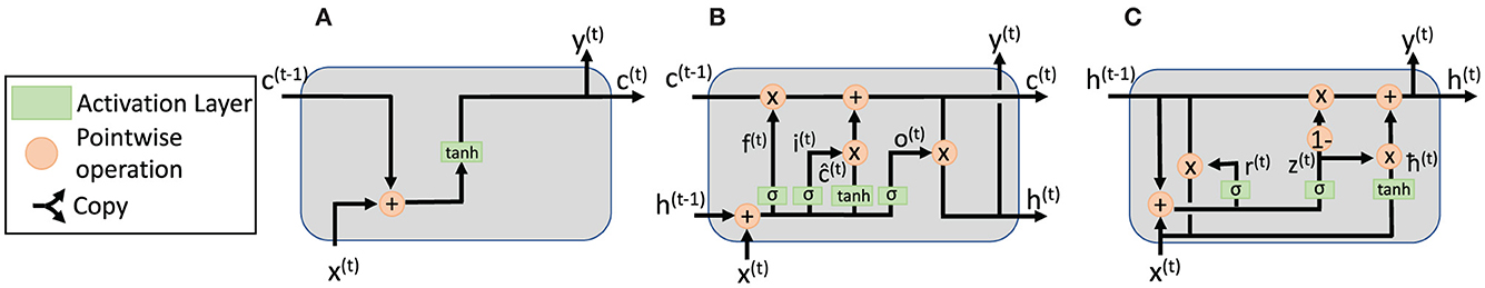
In theory, a basic RNN cell (cp. Figure 4A) should be capable of classifying long input sequences. However, in practice these cells suffer from vanishing and exploding gradient problems when longer sequences are processed and long-term relationships within EEG input data are relevant for signal analysis. To mitigate these problems, gated recurrent neural networks, most prominently long short-term memory (LSTM) and gated recurrent unit (GRU), have been proposed. These networks are considered among the most effective sequence modeling techniques today. While the basic RNN cell consists of a single layer with tanh activation, LSTM and GRU cells are more complex. Their key concept is different gates added to each of the states (cp. Figures 4B, C). These gates can learn what information is more or less relevant for further processing and regulate the flow of information through the network. A different approach that aims to overcome the problems of gradient descent-based learning are echo state networks (ESN) that use randomly initialized reservoir weights and merely a non-iterative learning of the output weights.

Figure 4. Schematic representation of non-gated and gated RNN cells: (A) basic RNN cell without any gates that is also representative for the reservoir of an ESN, (B) gated LSTM cell, and (C) gated GRU cell.

2.3.2. Long short term memory

The LSTM cell (Hochreiter and Schmidhuber, 1997) consists of three gates that shall help to overcome the problem of vanishing and exploding gradients (cp. Figure 4B). The first gate within an LSTM cell is a forget gate f(t) computing what information is required in the current cell state:

f(t)=σ(Wfhh(t-1)+Wfxx(t)+bf),    (2)

where Wfh and Wfx are weight matrices, bf is the bias, h(t−1) is the previous hidden state, and x(t) is the current input value. The output passes a sigmoid activation function σ bounded between 1, i.e., information is fully required, and 0, i.e., information is unnecessary. The second gate is the update gate i(t). It controls how much of the current input is considered when computing the new cell state:

c^(t)=tanh(Wchh(t-1)+Wcxx(t)+bc)i(t)=σ(Wihh(t-1)+Wixx(t)+bi)c(t)=(f(t)*c(t-1))+(i(t)*c^(t)),    (3)

where c^(t) refers to the tanh activated input at time step t. Analogous to the forget gate, the gate uses a sigmoid function which determines the importance of the respective information as i(t). The new cell state c(t) then becomes the combination of the information passing through the forget and the input gate, respectively. Finally, the output gate o(t) controls which information of the cell state is incorporated into the cell's current output y(t) and hidden state ht, respectively:

o(t)=σ(Wohh(t-1)+Woxx(t)+bo)y(t)=o(t)*tanh(c(t)).    (4) 2.3.3. Gated recurrent units

The GRU cell (Chung et al., 2014) was introduced in 2014 and is a simplification of the LSTM cell. The idea is to combine forget gate and input gate into a single relevance gate r(t) (cp. Figure 4C). By combining them, one weight matrix can be neglected, the cell state and hidden state are merged together, and the GRU cell is therefore supposed to be faster to train. Analogous to the LSTM cell described above, the state of the relevance gate r(t), the state of the updated gate z(t), and the hidden state h(t) are computed as follows:

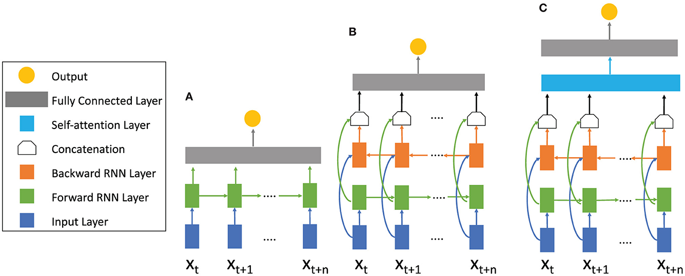
With the help of gates, GRU and LSTM (cp. Figure 5A) are supposed to be able to analyze longer sequences without being affected by vanishing gradients. Both variations are very popular for analyzing sequential data. While GRUs are more cost efficient due to fewer parameters, the LSTM contains more training capacity but requires more computational power and longer training time.

Figure 5. RNN architectures with different mechanisms. (A) Basic RNN architecture consisting of the input layer (blue) the RNN forward layer (green), and a fully connected layer (gray). The sequence is only calculated forward in time. (B) Bidirectional RNN architecture. In addition to the forward RNN layer a backward RNN (orange) layer is added. Information from the future and the past is calculated simultaneously and concatenated, summed, multiplied or averaged afterwards. (C) Attention Bidirectional RNN architecture. After the forward and backward calculations have been concatenated, an attention layer (blue) is used to pay attention to important sections of the sequence. For different RNN topologies like LSTM and GRU the cells within the forward and backward layer differ (see Figure 4).

2.3.4. Echo state networks

An alternative approach to potentially overcome the problems of gradient descent-based training is the non-iteratively trained echo state networks (ESN) (Jaeger, 2001). ESNs are a prominent RNN architecture that realize the reservoir computing paradigm (Verstraeten et al., 2007). An ESN consists of three core layers: the input layer, the reservoir layer, and the output layer. Only the weights of the output layer are trained. All other weights are typically randomly initialized from a uniform distribution, i.e., those of the input layer Whx∈ℝNres×Nin and those of the reservoir layer Whh∈ℝNres×Nres. A reservoir layer can be considered as a simplified RNN cell without most of the trainable parameters (cp. Figure 4A) and is denoted as:

h(t)=γ·h(t-1)+(1-γ)f(Whxx(t)+Whhh(t-1)),    (6)

where x(t) ∈ ℝNin is the input, h(t−1) ∈ ℝNres is the previous cell state, f(·) is an activation function, typically tanh, and γ is the leakage rate that determines how much of the ESN's previous hidden states is added to compute the new hidden state h(t). During the learning phase, a single training sequence ST with length T is utilized to compute the respective hidden states . The learning phase of an ESN is separated in two steps. First an initialization phase is done whereby the states are discarded, but the activation for each respective neuron is initialized (Jaeger, 2001). This process is often referred to as the washout phase (Malik et al., 2016). Second is the training phase, where the previous hidden states are added to the current hidden states, in relation to the leakage rate γ. The resulting matrix H ∈ ℝNres×T, which is based on the hidden states, is then mapped to the expected outputs Y ∈ ℝNout×T via a linear regression with y(t)=Wyh·h(t) according to:

Wyh=YH(HHT+βINr)-1,    (7)

with β as regularization coefficient and INr as unity matrix. For classification tasks, we train a reservoir for each class c within the dataset. We call this an ensemble of predictors, where each predictor processes the input file, and the class is chosen based on the predictor with the smallest error. For evaluation, each sample is processed by each predictor and is assigned to the class with the lowest prediction error (Forney et al., 2015).

2.3.5. Bidirectional architecture

In some applications, it can be helpful to process a sequence's previous as well as future information simultaneously. That is the concept of a bidirectional RNN combining two RNN layers, one for processing input data in a forward manner and one for processing input data in a reverse manner (Schuster and Paliwal, 1997) (cp. Figure 5B). The outputs of both layers are concatenated and eventually processed by a fully connected layer. This architectural approach is applicable for any RNN cell and has often been demonstrated to improve network performance when processing complex sequences in general (Huang et al., 2015; Yin et al., 2017) and to analyze EEG data (Ni et al., 2017; Chen et al., 2019). Ogawa et al. (2018) found that a bidirectional architecture improves accuracy in comparison to a basic RNN model by 1.1% for video classification based on the user's favors.

2.3.6. Attention

The attention mechanism is an imitation of human behavior. Rather than considering the entire previous input when computing the next output, a network learns which previously computed hidden states are beneficial to compute an output for a given new input. This approach is also applicable to any RNN cell and even to feed-forward networks as we will discuss in the next subsection. Attention computes the relation between the current input x(t) and previous inputs represented as hidden states with the help of an attention layer (Bahdanau et al., 2014; Cheng et al., 2016) (cp. Figure 5C):

ai(t)=vTtanh(Whhi+Wxx(t)+Wh~h~(t-1))si(t)=exp(ait)∑i′=1nexp(ai′t).

The attention calculation results in a distribution of probabilities of the previous values. With the probability distribution sit, an adaptive summary vector can be calculated. Cheng et al. (2016) proposes to replace the previous hidden state h(t−1) used in Equations (2)–(4) by a cell and hidden memory tape c~(t) and h~(t):

h~(t)=∑i=1t-1sit·hic~(t)=∑i=1t-1sit·ci.

The cell and hidden memory tape contain all the previous cell and hidden states and , respectively. Attention allows the network to give certain previous hidden states more weight in generating the current output than others. Thereby, rather than utilizing a single hidden state h(t−1) the network gains access to all previously processed hidden states and can weigh their importance.

2.4. Feed-forward networks

In contrast to recurrent neural networks, feed-forward networks like multilayer perceptrons (MLPs) and convolutional neural networks (CNNs) do not have any feedback connections between the output of a neuron and its input, i.e., input information x passes a series of operations and only influences the network's current output y. Traditional feed-forward networks were therefore not well suited to analyze time series data. Due to their non-recurrent nature, temporal dependencies could not be modeled well and extending the input size toward longer sequences became prohibitively expansive due to an exponentially growing number of parameters. However, there are more recent architectural concepts to overcome these limitations of FFNs in sequence processing, while preserving their benefits over RNNs, i.e., parallelizable training and being less prone to vanishing and exploding gradients. Below, we discuss three fundamental approaches for applying feed-forward architectures to time series data classification.

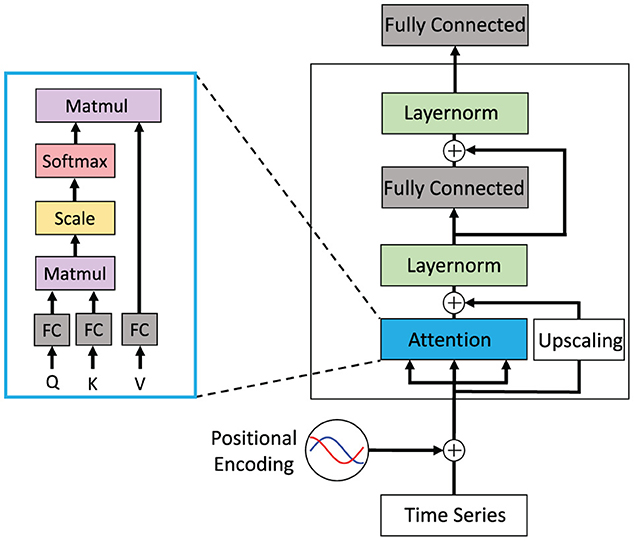
2.4.1. Transformer

The feed-forward Transformer architecture makes extensive use of the attention concept. It has been demonstrated to achieve superior results especially in the field of natural language processing (NLP) in recent years (Vaswani et al., 2017). Each block of the Transformer consists of an attention layer, a fully connected layer, and a final classification layer. Residual connections are added around the attention and fully connected layer followed by a layer normalization (cp. Figure 6). The attention mechanism is implemented as a multiplication of the input with three different weight matrices WQx, WKx, WVx and computed as:

α(Q,K,V)=s(Q·KTdk)V,    (8)

with Q, K, and V as Query, Key, and Value, respectively. The scaling factor is denoted as dk and the Softmax function as s(·). For solving NLP problems, such as machine translation, the Transformer typically follows an encoder-decoder structure (Vaswani et al., 2017). For classification problems only the encoder without the decoder part is used since only a single output conveying the classification result is required. Therefore, the model will be referred to as Transformer-Encoder in the rest of the paper.

Figure 6. Conceptual view of a Transformer block that shows a single attention layer that is typically realized as multiple attention heads. This Transformer block may be stacked multiple times and may be arranged in an encoder-decoder architecture with attention layers spanning across encoder and decoder. Figure replicated from Vaswani et al. (2017).

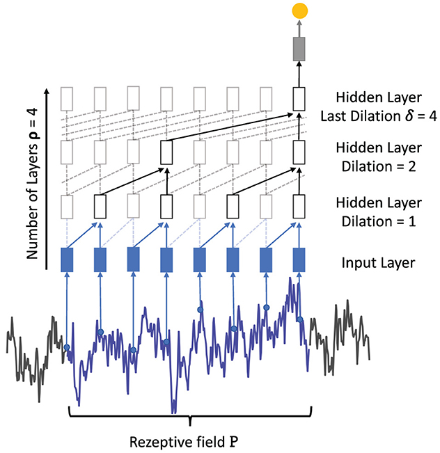
2.4.2. Temporal convolutional network

An alternative feed-forward architecture for the analysis of sequential data is the temporal 1D convolutional network (TCN) that is based on two key concepts (Bai et al., 2018). First, causal convolutions keep the temporal relationship between inputs, i.e., the input at time xt can only be convolved with an input of xt−n. Second, since a fully convolutional architecture would exponentially grow in depth with an increasing input length, dilated convolutions (Oord et al., 2016; Bai et al., 2018) are proposed and filter over larger input windows with a defined number of input are being skipped. Figure 7 illustrates the dilated convolutions concept where the first hidden layer convolves each two successive input values while the second hidden layer convolves two inputs but skips the intermediate one. The dilation rate δi increases exponentially with each hidden layer added to the network, starting with a dilation rate of 1. The number of TCN layers can therefore be derived by calculating the logarithm of the maximum dilation rate log2(dimax). Due to the dilation concept, TCNs are theoretically able to process sequences of any length without facing the problem of vanishing or exploding gradients. The amount of dilation per convolutional layer influences the receptive field P of a network calculated as:

P=1+(λ-1)·χ·∑iδi,    (9)

where χ is the number of TCN blocks, λ is the filter length, and δi is the dilation rate of the respective hidden layer. The example in Figure 7 consists of one TCN block, the last dilation is denoted as 4 and the filter size was set to 2. Using Equation (9) for dilated convolutions results in a receptive field of length 8. Without the use of dilated convolutions, the length of the receptive field would be 5 with the same amount of parameters. The TCN has been evaluated against LSTM and GRU on common sequence modeling datasets and demonstrated comparable and often better performance across the various tasks (Bai et al., 2018).

Figure 7. Visualization of a single TCN block χ for time series classification. Each time step of the time series is taken as input (for better visibility some points are removed from the example). With a filter size λ = 2, two samples are convolved, respectively. In the following hidden layers, the dilation ∈ [1,2,4] with a maximum dilation δ = 4 skips several samples and increases the length of the receptive field.

2.4.3. Extreme learning machines

Huang et al. (2004) proposed the extreme learning machine (ELM)