NeuroSuites: An online platform for running neuroscience, statistical, and machine learning tools

1. Introduction

There is a vast amount of data available today, and consequently, various software exists that aims to transform data into new knowledge. In particular, the analysis of neuroscience data can be especially complex, as some of these datasets (such as those from microarrays) can have tens of thousands of variables creating a need to develop powerful and efficient tools to handle the high dimensionality of these problems.

This motivated the development of NeuroSuites, a web application platform with numerous tools to help data scientists, and in particular neuroscientists, use specialized software to handle problems in their application domain. This platform is specifically designed to manage large-scale problems, which are common in some neuroscience fields.

In NeuroSuites we can find different parts related to a specific tool or set of processing tools, with emphasis on the field of neuroscience, such as morphological reconstructions and visualization of microscopy data. However, many other tools have a more generic aim and can also be used by data scientists from other research fields. In addition, no software installation is required on the computer, since it is designed as a web application, and all algorithms are executed on the backend of the deployed server, rather than requiring local computers with a large computational capacity to run the experiments. The web access is open and can be consulted from different devices as a result of its responsive web design.

The paper is organized as follows. In Section 2, we compare our platform with other currently available software, highlighting its main strengths compared to its competitors. This comparison will help us identify the most convenient type of users on our platform. Section 3 analyzes how NeuroSuites is implemented by reviewing the main technologies that make up its architecture. We also describe the services available on the platform and the main workflow when selecting a data source to use for a software tool. Section 4 focuses on the use of applications specifically oriented to neuroscience, where depending on the application, a previous selection of neuron reconstructions by the user may be needed. In Section 5 we present statistical tools aimed at exploratory data analysis and finding insights from this dataset, both with discrete and continuous variables. Section 6 focuses on the machine learning part of NeuroSuites, including various data preprocessing techniques, available supervised or unsupervised learning algorithms, and Bayesian networks. Finally, Section 7 concludes the paper with the main features of NeuroSuites and its great potential as an online platform. Possible improvements for future work are also discussed, such as implementing new tools in the platform.

2. Background

NeuroSuites is targeted at neuroscientists and any type of user who is seeking to perform data analysis quickly and easily through the different tools available. Currently, we can find some platforms with similar purposes. We selected some of them identified in different web reviews of machine learning and statistical service providers. To do so, we carried out a web review process of different rankings, comparisons and analyzes. The popularity or size of the company maintaining the service was also one of the factors that we considered, together with the existing documentation and means of support.

Next, we highlight the main features of our selected options:

• BigML is a machine learning platform that provides a service for developers to build great applications and perform real-time predictions. It also enables users to be productive and efficient regardless of the device they are using. However, to obtain all its functionalities in addition to those offered in free mode, a user must pay a monthly fee to access it.

• The KNIME Analytics Platform (Berthold et al., 2009) is an enterprise-level analytics solution for data scientists that utilizes the power of the Eclipse platform and a set of other powerful extensions designed for machine learning and data mining. Some of the key features included are workflow differentiation, big data extensions, meta node linking, robust statistical analysis and data blending. Nevertheless, it requires prior installation depending on the operating system of the local machine and monthly financial outlay as there is no lasting free version available.

• RapidMiner (Hofmann and Klinkenberg, 2016) is a toolset that provides a centralized solution ensuring a seamless process from modeling to implementation. It works not only for predictive analytics, but also for application integration, data integration, statistics, machine learning and transformation. It has a free version as well as paid plans. The core of RapidMiner stays open source.

• Weka (Hall et al., 2009) is a software platform that features a collection of machine learning algorithms to run data mining tasks. It stands out for being free software and a rather minimalist interface, where algorithms can be applied directly to a dataset or called from its own Java code. It is also well suited for developing new machine learning schemes and performing statistical experiments on different datasets. It is necessary to download the application on our local machine, rather than having a web version at the moment.

• Azure Machine Learning Studio (Barnes, 2015) is a Microsoft-backed professional predictive analytics programming solution that enables users to create effective machine learning models, which can be easily delivered as services. Users have to drag and drop objects into the platform interface and use a number of cloud-based tools to interactively run their experiments. It has a free version and a paid subscription to obtain all possible functionalities.

• Orange (Demšar et al., 2013) is an open source software for data mining and machine learning. The user can visualize large data like data flows and variable flows. Orange supports hands-on training and visual illustrations of concepts from data science, useful for teaching. There is no installation needed if you download a portable version, extracting the data file and opening the shortcut in the corresponding folder.

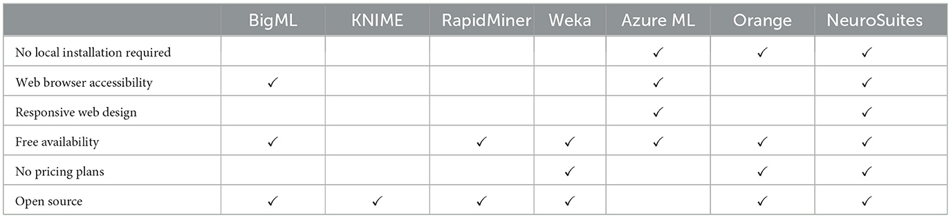
Table 1 shows a comparison of the main functionalities of each of the technologies described in this section. NeuroSuites (at the right most column) is a platform that encompasses several statistical and machine learning tools for neuroscience data. Moreover, there is no need to install any software on the local machine, as all algorithms run on a powerful stand-alone server. It is also important to note that it is hosted on a website where we developed all the necessary architecture to be able to deploy the different modules that make up NeuroSuites. Users can access it online simply through their web browsers, with no specific technical requirements on the users' end. There are no plans to include paid versions in our platform, and the complete code is accessible to everyone and can be found on GitLab. According to all of these functionalities, NeuroSuites is the most complete solution.

Table 1. Comparison between different machine learning software solutions.

3. NeuroSuites framework 3.1. NeuroSuites architecture

NeuroSuites aims to be a user-friendly application where everyone can use it, but regarding neuroscience, we intend to give data scientists and neuroscientists in particular the tools that they could need in a quick and easy way without installing several software tools in their computers. Furthermore, no computer science or programming knowledge is needed. Moreover, the software tries to comply with a responsive web design approach to make web pages render well on a variety of devices, contributing to the usability and satisfaction of the user experience.

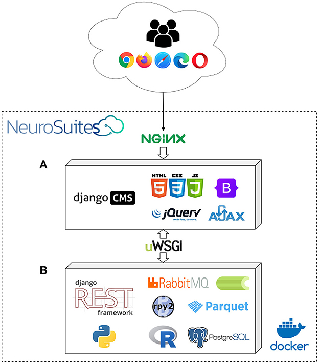
Next, we describe some important characteristics of the architecture of NeuroSuites (see Figure 1). It follows the model-view-controller architecture. When the workload is very intense in heavy operations, the number of workers will be increased and the queuing system will automatically distribute the workload. Thus, it can run heavy operations in the backend providing a quick and lightweight experience in the frontend. However, it is important to note that despite the implementation of this system, it is possible that certain operations will have a high execution time due to hardware limitations of the server itself on which our NeuroSuites instance is currently deployed.

Figure 1. NeuroSuites main architecture: frontend technologies (A) and backend technologies (B).

Users can access NeuroSuites through a web browser (Google Chrome, Firefox, Microsoft Edge, Opera...). The connection is made to the Nginx web server (Reese, 2008), which provides the entry point for web requests and acts as a load balancer in case the server has multiple instances running the web application.

For the frontend (Figure 1A) we use the Django CMS (George, 2015) to implement the different views, HTML, CSS with Bootstrap (Spurlock, 2013) and JavaScript with Jquery (Bibeault et al., 2015). On the client-side, the application creates asynchronous web applications using Ajax (Garrett, 2005) to send and retrieve data from a server asynchronously in the backend. To transmit the requests and responses from the frontend to the backend, we employ the uWSGI software which acts as a web server gateway interface to communicate with the backend.

For the backend (Figure 1B), we use Python and the Django REST framework (Rubio, 2017) to implement the different algorithms using some of Python's main optimized scientific libraries, highlighting NumPy (Harris et al., 2020), SciPy (Virtanen et al., 2020), or Scikit-learn (Pedregosa et al., 2011) among others. We also include bindings to the R programming language due to the wrappers provided with the rpy2 package. However, since standard HTTP requests and responses have temporal and computational limitations that prevent them from executing long-running tasks, we included a work queuing system using RabbitMQ (Dossot, 2014), which is a message-broker for long-term requests, and Celery, an open-source asynchronous task queue based on distributed message passing. In addition, to achieve greater memory efficiency, loaded datasets are stored internally on our server using the Apache Parquet format (Vohra, 2016), and to store the internal state of an application, the user's data session is stored in a PostgreSQL (Momjian, 2001) database connected to Django REST. It is important to note that the Django framework, compared to other alternatives with other programming languages, it allows an easy and fast deployment thanks to the use of Python libraries specific for machine learning.

All these technologies follow a modular architecture, where each fundamental component is isolated as a Docker microservice. Therefore, the system can be easily scalable horizontally and work as a whole given that platform as a service and its OS-level virtualization (the installed Docker container includes all the project images, so it can run without further configurations). In addition, multiple monitoring tools have been included (because the architecture became huge), such as logs to control the state of the hardware, task queues to check the current running tasks and possible issues, and several warnings on the backend side to provide us information about security problems and performance errors. Due to the computational limitations of our production server, we cannot provide more than one computing node. However, developers can install their own NeuroSuites instance and use this parallelization capability by deploying multiple computing nodes to run their Docker containers. We consider Docker to be a good solution for our project thanks to its rapid deployment, its simplicity in configuring new developments in each image facilitating the continuous integration of new functionalities. Finally, we use Git as a distributed version control; GitLab, in particular, as a service repository.

Finally, note that a user does not need to install anything to run the tools provided because everything is online. Additionally, when you finish a task, you can export and download your results to your own computer. Below, we focus on the capabilities and the steps needed to load data and run the different models.

3.2. Services available and general workflow

To provide an interoperable ecosystem, we designed a well-defined workflow consisting of first uploading the raw dataset and then selecting the desired tools to analyze it. Thus, different tools can be found on NeuroSuites, each referring to a specific set of processing units. In NeuroSuites, the main functionality is in the Services tab (Figure 2).

Figure 2. NeuroSuites' services tab. First, the data source to be used must be specified in step 1 (A). Then, an application can be selected from the menu on step 2 (B).

For the first step (Figure 2A), the user must select the data source. When selecting a data source, we present three different cases:

• Upload a dataset: we can “Upload a dataset” in csv or parquet format (there is available a “CSV dataset example from the Allen Brain Atlas”) or “Upload neuron reconstructions” in swc, dat, asc or json format.

• Continue without a dataset: if the user does not load any data source of his or her own, it is still possible to access some software tools (such as some neuro apps).

• Demo data: load a set of NeuroMorpho.org neurons to test all available tools in NeuroSuites. NeuroMorpho is a centrally curated inventory of digitally reconstructed neurons publicly accessible associated with peer-reviewed publications and created by George Mason University. You can browse their website, download a specific set of neurons and then upload the data in NeuroSuites.

Once we have the data source loaded in the platform, we are able to see a list of all the applications currently available in NeuroSuites. We can also group them according to different themes, such as neuroscience, general purpose or software with/without the required dataset (Figure 2B).

4. Neuroscience applications

After selecting the data that we are going to use, we have different options in regard to analyzing our data. Figure 3 shows all neuroscience tools available after previously selecting a data source.

Figure 3. Neuroscience applications in NeuroSuites: L-Measure (A), NeuroViewer (B), NeuroSTR (C), 3DBasalRM (D), GabaClassifier (E), 3DspineS (F), 3DSomaMS (G), 3DSynapsesSA (H), Dendritic arborisation simulation (I), and MultiMap (J).

4.1. Neuro apps with neurons required

Some applications are enabled only when we previously set the neurons we want to analyze. After that, in a new window, we can see an overview with a list of all neurons to analyze them one-by-one. When selecting a specific neuron, we can see some neuro app software tools that can be applied to the selected neurons to view them (bottom-up approach). Conversely, we can select a specific software tool from the NeuroSuites side menu and then apply it to our neurons (top-down approach).

For example, suppose that we select one neuron available in the overview (table with our set of neurons) using the demo data from NeuroMorpho. A new window can show more specific details about the neuron along with a number of software tools that can be applied to the selected neuron.

First, we can use the L-Measure (Figure 3A), a tool that allows researchers to extract quantitative morphological measurements from neuronal reconstructions (Scorcioni et al., 2008). Second, we can also use NeuroViewer (Figure 3B), a 3D neuron reconstruction visualization package. There are some camera, render and animation options, together with the possibility of setting the neurite values we want to reconstruct and plot from the selected neuron.

Moreover, we have 3DBasalRM (Figure 3C), a data-driven repair model that detects cut-points in the basal arborisation and then repairs them using a growth model learned from full 3D neuron reconstructions. Figure 4A shows the reconstruction of the 02a_pyramidal2aFI_CNG neuron with NeuroViewer using the demo data from NeuroMorpho. Then, Figure 4B shows the repaired neuron 02a_pyramidal2aFI_CNG after applying this model. Finally, it is possible to save these results in swc and json formats.

Figure 4. (A) 3D reconstruction of 02a_pyramidal2aFI_CNG neuron with NeuroViewer and (B) its repaired neuron using the 3DBasalRM tool. (C) NeuroSTR validator for 10 neurons selected from the demo data.

Another application available is NeuroSTR (Figure 3D), a neuroanatomy toolbox created in our lab that can read and process 3D neuron reconstructions in the most common file formats, offering a very large set of utilities to work with. For instance, we can check wether neurites are attached or not to the soma and some validators, such as a trifurcation on nodes that cannot have more than two descendants. Figure 4C shows the checks and validators for 10 neurons. The checks and validators available are the following: neurites are attached to soma, neuron has soma, planar neurite validation, basal dendrite count, strict apical dendrite count, strict axon count, trifurcation validator, linear branch validator, zero length segments validator, the length smaller than the radius validator, non-decreasing diameter validator, branch collision validator, and extreme angles validator. In addition, a format converter of reconstruction file translates it into swc or json (optionally, it tries to correct errors in the reconstruction and applies a simplification algorithm over the branches).

Finally, GabaClassifier (Figure 3E) can be used to classify a given interneuron morphology into one of the seven possible classes described in Markram et al. (2004). The output is a short string code representing the following possible class names: bitufted cell, chandelier cell, double bouquet cell, large basket cell, Martinotti cell, nest basket cell, and small basket cell.

It should be noted that all the tools described in this section, with the exception of L-Measure, have been developed in our laboratory.

4.2. Neuro apps without neurons required

In NeuroSuites, we can also access some tools that do not require prior data loading (all of them developed in our laboratory):

• 3DspineS (Figure 3F), a model-based clustering of dendritic spines from their 3D morphological features. Moreover, the clustering model also allows us to accurately simulate spines from human pyramidal neurons to suggest new hypotheses of the functional organization of these cells (Luengo-Sanchez et al., 2018).

• 3DSomaMS (Figure 3G), a software that provides a mathematical definition and an automatic segmentation method to delimit the neuronal soma due to its fuzzy definition, as there is no clear line demarcating the soma of a labeled neuron and the origin of dendrites and axon (Luengo-Sanchez et al., 2015).

• 3DSynapsesSA (Figure 3H), a tool designed to process and analyze patterns of the 3D spatial distribution of cortical synapses. It brings a variety of both innovative and well-known techniques from the spatial statistics (and more specifically, spatial point processes) field (Anton-Sanchez et al., 2017).

• Dendritic arborisation simulation (Figure 3I), a simulation for generating synthetic arbors of neurons with soma and dendrites (López-Cruz et al., 2011). These computational models are important for studying dendritic morphology and its role in brain function.

• MultiMap (Figure 3J), an extensible application to deal with large stacks of confocal microscopic images at different levels of resolutions (Varando et al., 2018). The possibility of creating regions of interest (of any shape and size) is a great advantage of the tool.

5. Statistical analysis

Next, the neuroscientist may be interested in descriptive and inferential statistics, given a dataset. We differentiate between discrete or continuous data to perform different statistical analyzes. Additionally, we distinguish between statistical calculations on a single variable (univariate statistics), and a multivariate analysis (multivariate statistics) where two or more variables are analyzed to determine their relationship. Several examples can be seen using a dataset from the Allen Human Brain Atlas dataset (Hawrylycz et al., 2012), available as demo data (Figure 2A) in NeuroSuites. These tools were developed using the rpy2 package for the use of statistical functions.

5.1. Statistical tools with categorical data

NeuroSuites has a side menu where a user can select statistics for discrete or continuous data. Several use cases for these options are introduced below. First, the number of rows and columns of our previously loaded dataset is indicated. Next, we can find two tabs, one for descriptive statistics and the other for inferential statistics.

In descriptive statistics, we can select the discrete or categorical variables we wish to visualize graphically in pie charts. For example, if we select neuron_reconstruction_type, the number and percentage of instances for each value or category of that variable are shown. In this case, the variable has three possible values: full, dendrite-only, and none. It is also possible to view this frequency distribution via tabular summary of data for a single variable. The tabular data can be downloaded in different file formats. Within the bivariate analysis, it is possible to display a stacked bar chart and a grouped bar chart on the selected variables instead of a single pie chart for one variable.

Regarding inferential statistics, we can estimate probability distribution parameters, both as confidence intervals and point estimations. After specifying the confidence level of the interval, the point estimation and interval estimation will be displayed. We can also visualize the plot of the Gaussian distribution for the sample mean (i.e., the proportion point estimate with their tabular stats).

It is also possible to perform statistical hypothesis tests, specifying the population proportion for the null hypothesis. In addition, it is also possible to compare two proportions from two independent populations. However, this type of McNemar's test is only possible with binary variables.

Finally, the distribution of the data can also be checked by either automatically finding the fittest distribution or by selecting only the distribution we want to check, all with a given significance level. Performing these tests, the χ2 statistic is used to calculate the goodness of fit. This test is not valid when the observed or expected frequencies in each category are too small (a typical rule of thumb is that all observed and expected frequencies should be at least 5).

5.2. Statistical tools with continuous data

Following a similar structure to that presented in the previous section, in this case, we can see other functionalities with continuous variables. If we select the continuous variables average_contraction and average_diameter, it is possible to have univariate plots, such as the histogram and the fitted probability density function, box plot and a scatter plot. In the case of performing bivariate statistics, we can obtain the Pearson, Kendall and Spearman correlation coefficients (Figure 5A), and visualize the scatter plot matrix together with its 2D histogram contour plot (Figure 5B).

Figure 5. Pearson, Kendall, and Spearman correlation coefficents (A) with a 2D histogram contour plot (B) for the variables average_contraction and average_diameter. Note their negative correlation.

We can perform analyzes with three or more variables. In that case, we can visualize a scatter bubble plot (Figure 6A) and a 3D scatter plot (Figure 6B) of the selected variables average_contraction, average_diameter and average_fragmentation.

Figure 6. (A) Scatter bubble plot and (B) 3D scatter plot with the variables average_contraction, average_diameter and average_fragmentation. (C) Radar chart and (D) Andrews plot with the same set of variables. (E) RadViz plot for the variables average_contraction, average_diameter, average_fragmentation, average_parent_daughter_ratio and avg_isi.

As an example where multiple variables are needed, suppose the data scientist is interesting in finding which observations are the most similar and those that are possibly outliers. The structure of the data has a high dimensionality, meaning that it is necessary to use different techniques to visualize as many dimensions as possible in a given graph. Figure 6C shows a radar chart to compare different variables in an easy way, Figure 6D is an Andrews plot to visualize and check the structure of the variables (possible groups), and Figure 6E a RadViz plot to visualize each variable around a circumference of a circle with normalized values. These plots use multiple selected variables (for the latter we use five variables for visualization purposes). We can also visualize all their probability density functions in the same plot, parallel coordinate plots, or Chernoff faces for multiple variables.

For categorical variables, we can also apply inferential statistics to continuous data. It is also possible to obtain point and confidence interval estimates. The variance estimate is Bessel-corrected (unbiased), and a Student's t-distribution is used to calculate the confidence interval for the expected mean of a variable that is assumed to follow a normal distribution (since the population variance is generally unknown). After selecting one or more variables and specifying a confidence level, graphs and tabular statistics appear in the web interface.

It is also possible to perform hypothesis testing in the same way as for categorical variables. To test the mean, we specify a given value of the population mean (null hypothesis), a variable from our dataset, and a significance level. After running the hypothesis test, we can see the hypothesis result with some statistical measures. We accept or reject the null hypothesis in favor of the alternative hypothesis, thus concluding the test. We can visualize the probability density function of the Student's t-distribution associated with the test statistic.

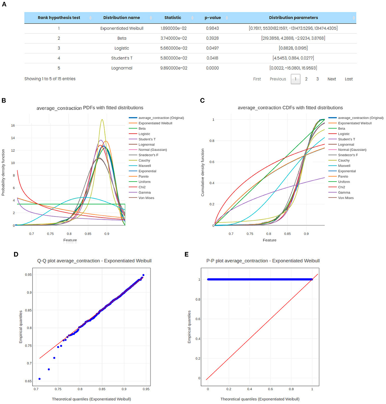
Finally, to check the distribution of the data, we can either automatically find the fittest distribution or set a null hypothesis test (e.g., data following a Gaussian distribution) and an alternative hypothesis test (e.g., data does not follow a Gaussian distribution). Figure 7 shows an example of the best distribution of a fixed and finite set of possible probability density functions for the variable average_contraction that was found using a significance level of 5%. Two goodness-of-fit measures are taken, the Akaike information criterion and the Kolmogorov-Smirnov test. The ranks of the different distributions are sorted in tabular form with some statistical measures (Figure 7A). In this case, the exponentiated Weibull is the fittest distribution, ranking first in the hypothesis ranking. Moreover, we can see the probability density function (Figure 7B) and the cumulative distribution function (Figure 7C), both with the fitted distributions. Finally, we can also see the Q-Q plot (Figure 7D) and the P-P plot (Figure 7E) comparing the probability distributions of our variable (empirical) with its fittest distribution (theoretical).

Figure 7. (A) Ranking of the fittest distributions using two goodness-of-fit measures, the Akaike information criterion and the Kolmogorov-Smirnov test. (B) Probability density functions with their fittest distributions. (C) Cumulative distribution functions with their fittest distributions. (D) Q-Q plot with the exponentiated Weibull distribution. (E) P-P plot with the exponentiated Weibull distribution. In all of these cases, we use the variable average_contraction and a significance level of 5%.

6. Machine learning

This section reviews some machine learning algorithms that can provide us with more insights into our dataset. The behavior in all windows is very similar; a user selects the data source differentiating the variables that are discrete or continuous, the multiple variables a user wants to analyze and, optionally, class variables when necessary.

Table 2 shows all the available machine learning algorithms available in NeuroSuites. Each tool selected in NeuroSuites has its own parameters that can be configured in the same tab. Once the algorithm and the desired parameters have been selected, the results obtained are displayed in a new tab in tabular and graphical form, although it varies depending on the tool we are handling.

Table 2. Machine learning tools in NeuroSuites.

6.1. Data preprocessing techniques

We can handle missing values via row deletion or by an imputation process to replace missing data with the imputed values (such as the mean substitution technique). It is also possible to remove constant irrelevant variables. It is remarkable that for all these options, users have listboxes and checkboxes to select the desired functionality.

Another option available is normalization, using well-known techniques such as the min-max variable scaling (used to bring all values into the range [0, 1]). Moreover, there are some discretisation methods of continuous values, such as the equal-frequency binning or Fayyad & Irani's algorithm (Fayyad and Irani, 1993).

As part of the data preprocessing, we can apply a filter feature subset selection algorithm, such as chi squared, mutual information or ANOVA F-test, with their specific filter criteria (selecting the k best features, a selected percentile of features or the features that pass a family-wise error test).

Additionally, the techniques of dimensionality reduction to obtain a lower dimension dataset are sparse and nonlinear principal component analysis (PCA), independent component analysis (ICA), t-SNE (Van der Maaten and Hinton, 2008) and multidimensional scaling. A user can also use these methods either before or after the feature subset selection, and specify a desired number of dimensions.

6.2. Unsupervised classification

It is useful to see some plots when handling clustering problems. In this sense, NeuroSuites has the implementation of some non-probabilistic clustering algorithms (see Table 2). Figure 8 shows the dendrogram after applying the agglomerative hierarchical clustering algorithm to the variables average_contraction, average_diameter, average_fragmentation, average_parent_daughter_ratio and average_isi. In this case, the number of clusters is 16, using Ward's linkage and Euclidean distance. A user can also set a distance to cut the dendrogram tree with a horizontal line without intersecting the merging point.

Figure 8. Agglomerative hierarchical clustering dendrogram for instances using Ward's linkage and Euclidean distance with the variables average_contraction, average_diameter, average_fragmentation, average_parent_daughter_ratio and average_isi.

The user can modify the available configurations, and choose other types of clustering algorithms such as partitional clustering using K-means, DBSCAN (Ester et al., 1996) or spectral clustering. Suppose we are going to use the K-means algorithm for the same variables mentioned above. We can view the elbow method plot to help determine the number of clusters (Figure 9A), a clustering plot with its instances on a 2D map (Figure 9B) and the overall tabular data with cluster centroids (Figure 9C).

Figure 9. K-means clustering algorithm with the variables average_contraction, average_diameter, average_fragmentation, average_parent_daughter_ratio and average_isi. (A) Elbow method plot suggesting five clusters. (B) Clustering plot on a 2D map using PCA. (C) Tabular data with the cluster centroids.

6.3. Bayesian networks

For this type of probabilistic graphical model, we use BayeSuites (embedded within NeuroSuites), a web framework developed in our lab for massive Bayesian networks focused on neuroscience (Michiels et al., 2021). Once the desired variables have been selected, we can learn the structure graph and the parameters from a dataset by selecting a structure and parameter learning algorithm. Table 3 shows the structure and parameter learning algorithms currently available in NeuroSuites. Some of these algorithms have been coded internally (backend NeuroSuites) since they are novel contributions, while others have been directly imported from external libraries, adapting the functions so that they can run on the selected data. The graph obtained after running the learning algorithm is displayed in the viewer.

Table 3. Structure and parameter learning algorithms for Bayesian networks in NeuroSuites (and BayeSuites).

When visualizing a Bayesian network, there are several layouts (tree-based, force-directed, circular, grid, image) and viewing options (zooming in/out, scale and filtering options). Moreover, a user can also create groups of nodes or highlight the nodes of the Markov blanket of a given node or its parents or children. An example of a (Gaussian) Bayesian network representing a gene regulatory network (GRN) of the full human genome (Hawrylycz et al., 2012) is shown in Figure 10A, where we select the ForceAtlas2 layout (Jacomy et al., 2014) and the Louvain algorithm (Blondel et al., 2008) to generate groups of nodes colored for community detection. In addition, a user can make some probabilistic queries, introduce the evidence to perform inference, and check the d-separation between three groups of nodes (Koller and Friedman, 2009). Figure 10B shows a selection of one random node associated with schizophrenia disease subset of nodes. After visualizing the node parameters (mean and standard deviation) and transforming it to an evidence node (with a value fixed), then a user can start the inference process and see the resulting new (Gaussian) distribution.

Figure 10. (A) BayeSuites viewer example of the structure of a Bayesian network representing a large GRN with the ForceAtlas2 force-directed layout and using the Louvain algorithm to generate groups of nodes colored for communities detection. (B) Parameter visualization and inference for a node (KIF17) associated with the schizophrenia disease subset of nodes. Taken from Michiels et al. (2021).

6.4. Supervised classification

When a class variable is present, many algorithms are available in NeuroSuites (see Table 2). First, it is possible to run some Bayesian classifiers (Bielza and Larrañaga, 2014) already coded using the bnlearn package, such as the naive Bayes and the tree augmented naive Bayes (TAN) classifiers (Friedman et al., 1997). These classifiers are based on Bayesian networks, standing out for their interpretability and the existence of efficient algorithms for learning and classification tasks.

Classification tree algorithms have been implemented on the backend using the Scikit-learn library (built on NumPy, SciPy, and Matplotlib), together with Graphviz for frontend visualization of graphs representing structural information. The classification tree algorithm used is an optimized version of the classification and regression trees (CART) algorithm, similar to the C4.5 algorithm, with a 10-fold stratified cross-validation. It is possible to modify other options, such as the criterion, to measure the quality of a split (Gini index or entropy-based), the strategy used to choose the split at each node (best or random) or the maximum depth of the tree. Moreover, a user can visualize a text report showing the rules of a decision tree with their main performance measures, such as accuracy, sensitivity, specificity or F1-measure.

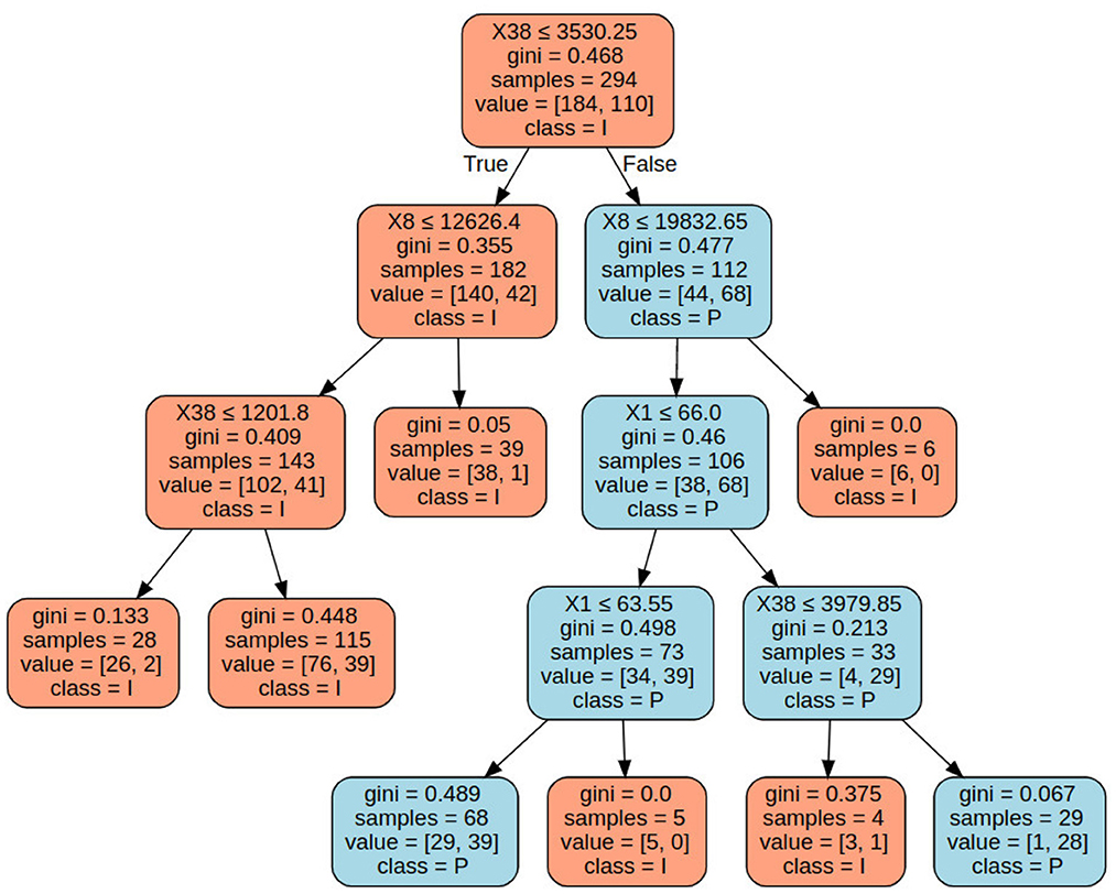
To illustrate some examples, the dataset we selected comes from Bielza and Larrañaga (2020), which seeks to distinguish pyramidal cells (class P) from interneurons (class I) in the mouse neocortex. Figure 11 shows the classification tree for the selected subset of three variables: X1 (somatic perimeter), X8 (total axon length) and X38 (total dendritic length), all measured in μm. As we go deeper into the classification tree toward the leaf nodes, we obtain a more precise classification according to the new rules for moving toward one node or another. In this example, if the instance is classified as interneuron, the node is colored orange; if it is classified as a pyramidal cell, the node is colored blue. Thus, for example, if the value of X38 ≤ 3, 580.25, the classification tree will classify the instance as an interneuron (class I). Moreover, if the value of. X8>12, 626.4, we can see that the tree has correctly classified almost all the samples (low Gini impurity).

Figure 11. Classification tree yielded by the CART algorithm for predictor variables X1 (somatic perimeter), X8 (total axon length) and X38 (total dendritic length), using the Gini criterion and a 10-fold stratified cross-validation. In each node, a user can see the following: attribute test, samples, value (how many samples belong to each category) and the class classified up to that depth level.

For the k-nearest neighbors (k-NN) algorithm, we can specify parameters, such as the number of neighbors we want to use or the weight function used in prediction, which can be uniform (all points in each neighborhood are weighted equally) or based on the distance (weighting points by the inverse of their distance to the target point).

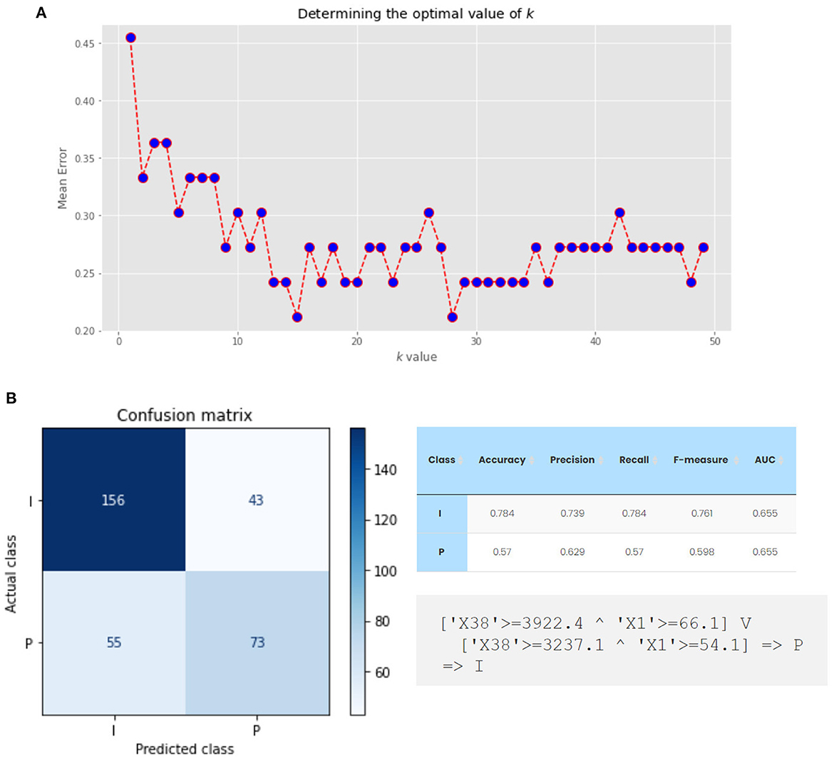
NeuroSuites can determine the optimal value of k at a glance. Figure 12 shows an example of the mean error for each value of k after applying the k-NN algorithm. In this case, we specified a holdout scheme for estimating the different performance metrics, with 90% of the data for training and the remaining 10% for testing. It can be seen how from k = 13, we can obtain good results with a mean error of less than 0.25. For a high value of k, it seems that the mean error worsens.

Figure 12. (A) Mean error for each k value of the k-NN algorithm for the variables X1 (somatic perimeter), X8 (total axon length) and X38 (total dendritic length) as predictors, using uniform weights and a train-test split scheme of 90%-10%. (B) RIPPER algorithm output for variables X1 (somatic perimeter), X8 (total axon length) and X38 (total dendritic length) as predictors, with their confusion matrix (left), performance evaluation metrics (top right) and ruleset (bottom right).

The implementation of support vector machines (SVMs) is based on LIBSVM (Chang and Lin, 2011). For these models, we can specify that the kernel is linear (for the linear SVM case) or nonlinear, including the polynomial (degree parameter required), radial basis function, and sigmoid as different options. As with the rest of the supervised models, after running the algorithm, one can see the main performance measures with the confusion matrix.

It is also possible to run the RIPPER rule induction algorithm to obtain the rules. This type of algorithm together with classification trees, can be of great help to data scientists when making decisions as they are algorithms with high interpretability, following the current trend of explainable artificial intelligence (Gunning et al., 2019) as opposed to other types of black box models, such as deep neural networks.

The RIPPER algorithm available in NeuroSuites is based on the wittgenstein package, written in Python. Figure 12 shows an example for the same dataset we are using thus far with the output rules, their main performance measures and the confusion matrix for this binary classification example. In this case, the rules shown consider the X38 and X1 variables (^ represents the logical conjunction, whereas V denotes the logical disjunction). If the rules of the variables are met, it is classified as a pyramidal cell (⇒ P); otherwise, it is an interneuron (⇒ I).

Bayes' rule is used in some classifiers, such as linear discriminant analysis (LDA) and quadratic discriminant analysis (QDA), creating decision boundaries of different complexity to classify the new data. LDA uses a singular value decomposition as a solver. Both models fit a Gaussian probability density function for each class value. Finally, we can run a logistic regression classifier. L2 regularization is applied by default, adding an L2 penalty term.

6.5. Multidimensional classifiers

There are some multidimensional classifiers currently available in our platform, where the aim is to predict more than one class variable at the same time. With this type of classifier, we included learning methods of the two main approaches: (1) problem transformation methods, where the multi-label problem is turned into many single-label problems; and (2) algorithm adaptation methods, where uni-dimensional supervised classification techniques are adapted to directly manage multi-label (when all class variables are binary) or multidimensional data.

All of these available classifiers are categorized by their method type and function implementation using Sklearn as backend. After defining the target classes and, optionally, whether to use a number of k-folds for cross-validation, depending on the type of problem transformation, users are able to set different parameters. For the case of transforming the problem to binary or multi-class classification, a user can specify the classification algorithm with a few hyperparameters. The following classifiers are currently available: k-NN, classification tree, SVM, LDA, QDA, logistic regression and naive Bayes. Once selected, their performance evaluation measures adapted to multidimensional classification are shown.

7. Conclusions

In this paper we presented NeuroSuites, a powerful open access web platform with a wide range of software tools devoted to statistics and machine learning. It also has several applications and tools specifically dedicated to the neuroscience domain, as well as more general ones oriented to help any data scientist in his or her application domain.

We developed the entire web interface to provide the best user experience for devices connecting to the domain on which NeuroSuites is deployed. In addition to neuroscience applications, it is possible to perform statistical analysis and machine learning modeling for large amounts of data without being limited by the computational capacity of personal devices.

Finally, we would like to emphasize our intention to continue expanding the list of available software tools, as well as improving the platform interface according to user demands. The maintenance of the web and the correct functioning of the servers are something important that we will continue to consider to reinforce the robustness of the platform. The architecture has been designed to be able to easily implement future updates and improvements on the different tools.

In future work, we plan to implement probabilistic clustering algorithms to complement what we already have in NeuroSuites. Furthermore, we are also considering including a section on artificial neural networks to visualize the network structure and train different deep learning models, although we think that the interpretability of the model has a greater relevance in the field of neuroscience and post-hoc explainability issues should also be incorporated.

Data availability statement

Publicly available datasets were analyzed in this study. This data can be found here: https://gitlab.com/mmichiels/neurosuite; https://github.com/ComputationalIntelligenceGroup.

Author contributions

JLM-R worked on the development of the platform and the first version of the manuscript. PL and CB have conceived the project by helping in its conceptualization and supervision of the manuscript. All authors contributed to the article and approved the submitted version.

Funding

This project had received funding from the European Union's Horizon 2020 Framework Programme for Research and Innovation under Specific Grant Agreement No. 785907 (HBP SGA3) and from the Spanish Ministry of Science and Innovation through the PID2019-109247GB-I00 project.

Conflict of interest

The authors declare that the research was conducted in the absence of any commercial or financial relationships that could be construed as a potential conflict of interest.

Publisher's note

All claims expressed in this article are solely those of the authors and do not necessarily represent those of their affiliated organizations, or those of the publisher, the editors and the reviewers. Any product that may be evaluated in this article, or claim that may be made by its manufacturer, is not guaranteed or endorsed by the publisher.

Footnotes References

Aliferis, C. F., Tsamardinos, I., and Statnikov, A. (2003). “HITON: a novel Markov blanket algorithm for optimal variable selection,” in AMIA Annual Symposium Proceedings, Vol. 2003 (Washington, DC: American Medical Informatics Association), 21.

PubMed Abstract | Google Scholar

Anton-Sanchez, L., Larrañaga, P., Benavides-Piccione, R., Fernaud-Espinosa, I., DeFelipe, J., and Bielza, C. (2017). Three-dimensional spatial modeling of spines along dendritic networks in human cortical pyramidal neurons. PLoS ONE 12, e0180400. doi: 10.1371/journal.pone.0180400

PubMed Abstract | CrossRef Full Text | Google Scholar

Aragam, B., Gu, J., and Zhou, Q. (2019). Learning large-scale Bayesian networks with the sparsebn package. J. Stat. Softw. 91, e12776. doi: 10.18637/jss.v091.i11

CrossRef Full Text | Google Scholar

Barnes, J. (2015). Azure Machine Learning. Redmond, WA: Microsoft Press.

Google Scholar

Bernaola, N., Michiels, M., Larrañaga, P., and Bielza, C. (2020). Learning massive interpretable gene regulatory networks of the human brain by merging Bayesian networks. bioRxiv. doi: 10.1101/2020.02.05.935007

CrossRef Full Text | Google Scholar

Berthold, M. R., Cebron, N., Dill, F., Gabriel, T. R., Kötter, T., Meinl, T., et al. (2009). KNIME-the Konstanz information miner: version 2.0 and beyond. ACM SIGKDD Explorat. Newslett. 11, 26–31. doi: 10.1145/1656274.1656280