Training data for the post-reconstruction deep learning models were obtained by randomly sampling 50 stress and rest gated MPS studies (total of 100 acquisitions) from Lahti Central Hospital’s database. The training data included studies reported both as normal and abnormal and were supposed to reflect the entire MPS patient material at our centre. The ethics committee of Joint Authority for Päijät-Häme Social and Health Care has granted approval for this study. The studies were acquired using a 1-day protocol, whereby a vasodilator-induced stress study was performed in the morning and a nitrate-enhanced rest study 3 h later in the afternoon. Weight-based dosing of 99mTc-tetrofosmin was used. The activity of the stress injection was approximately 250 MBq and rest injection 750 MBq. Studies were acquired either with Siemens Symbia T or Siemens Intevo Bold using 90-degree angle between the detectors, 64 projections over 180 degrees rotation, 128 × 128 matrix, 4.8 mm pixel size, 40 s acquisition per projection and 8 cardiac gated frames per R-R interval. The quality of cardiac gating was monitored during acquisition time. Only successfully gated studies were used. After each SPECT study, a low-dose CT was performed using 130 kV tube voltage, 17 mAs tube current and 5.0 mm slice thickness to obtain the attenuation map.

Reduced acquisition time datasets were simulated by summing different numbers of cardiac gates. Full time, half time, three-eighths time and quarter time acquisition data were generated by summing all, half, three and two cardiac gated frames per projection, respectively. The indices (1–8) of the cardiac gates selected for summing for the reduced time acquisitions were randomly sampled for each projection.

All the studies were reconstructed using HERMES Medical Solutions’ (Stockholm, Sweden) HybridRecon ordered subsets expectation maximization (OSEM) algorithm with collimator response, attenuation and Monte Carlo-based scatter modelling [11]. The number of subsets was set to 16, number of iterations 5 and 3D Gaussian post-filter full width at half maximum to 1.25 cm. After reconstruction, images were cropped into 32 × 32 × 32 patches with stride of 8. Image cropping increased the size of training dataset and reduced the memory requirements of the DL model training. Stress and rest patches obtained with half time, three-eighths time and quarter time were all pooled together after cropping and then used to train the DL models with the matching full time patches. Approximately 50,000 patches were used to train each DL model and only one DL model for each DL strategy (CNN, RES, UNET and cGAN) was generated.

Four different DL-based denoising models were compared. The structure of the models is shown in Fig. 1 in more detail. The CNN model consisted of 8 layers each with 8 filters (3 × 3 × 3 filters and rectified linear unit (Relu) as activation function) and skip connections between the layers. In RES, the convolution blocks of the CNN model were replaced by residual units also shown in Fig. 1. The third model was UNET network. In UNET, the reduced acquisition time patch is first mapped to a latent representation of the input patch in a series of encoding layers. Each resolution level of the encoding path consisted of two convolutional operations followed by Relu (UNET block in Fig. 1). Between resolution levels, the spatial size of the patches is halved using maximum pooling (maxpool) operation. The decoding part, which is used to reconstruct the latent representation into full acquisition time version of the original patch, has similar resolution levels as the encoding path and the patch is up-sampled using transposed convolution between the levels. Skip connections were also used with UNET. CNN, RES and UNET used L2-norm as cost function.

DL models. The number under the blocks presents the patch size (upper number) and number of filters (lower number). Noisy 32 × 32 × 32 patches cropped from reduced acquisition time OSEM images were used as model input and model gave denoised 32 × 32 × 32 patches as output. Output patches were later combined using weighted averaging to produce images at the original reconstruction matrix size

The fourth model was cGAN, which consists of two networks. First network, called generator network, whose structure here is similar to UNET, produces denoised versions of the reduced acquisition time inputs. The second network, called the discriminator, tries to determine if the input is a generator-denoised patch or a true full time patch. The discriminator consisted of 4 convolutional layers, where the image size was reduced with 4 × 4 × 4 stride 2 convolution, followed by a fully connected layer. Leaky Relu (LRelu) was used as an activation function for all other layers except for the last where sigmoid function was used. The cost function for cGAN was a combination of L2-norm for the generator and binary cross-entropy for the discriminator.

The model parameters (number of layers and filters) for all the models were determined by testing different layer and filter number combinations using one-fifth of the training data. Visual image quality and root mean square error with the full time image were used the grade the layer and filter number combinations. The models were generated and trained using Python (version 3.6.8) and Tensorflow (version 2.4). Adam optimizer was applied using the default settings. One hundred epochs with a batch size of 32 were used.

When the DL models were later applied to test data also the test data were cropped into 32 × 32 × 32 patches with stride of 8. The overlapping 32 × 32 × 32 patches were combined after denoising using weighted averaging, where the value of each patch voxel was weighted by the inverse distance of the patch voxel from the patch centre before it was added to the final denoised image. Similar approach was used in [12].

Test data for the DL models were obtained by searching Lahti Central Hospital’s database for stress and rest MPS cases, which the reporting physicians had reported as normal without any visible SPECT perfusion defects. These studies were also not part of the DL training data. Forty-three stress and rest studies were selected. These data were acquired using the same cameras and parameters as the training data. These normal studies were divided into two sets. The first set consisted of 20 studies (20 stress studies and 20 rest studies), which were used to assess the noise level and SSIM and were also used to form studies with known artificial defects. The second set consisted of 23 studies (23 stress studies and 23 rest studies), which were used to build normal databases to assess perfusion detection performance.

For noise level and SSIM assessment, the cardiac gates for the 20 normal studies were summed and full, half and quarter time acquisition data were generated as explained earlier. (Three-eighths time acquisition time data were not used for testing.) All the generated studies were reconstructed using HERMES Medical Solution’s HybridRecon with the same settings that were applied during model training. The four DL-based models were used to denoise the half and quarter time images after reconstruction. Full time, half time and quarter time OSEM without denoising was used as a reference for the DL models.

Perfusion defect detection performance assessment required studies with known defects. Test cases with artificial defects were generated by first reconstructing the 20 stress and rest normal studies using HERMES Medical Solution’s HybridRecon with the same settings that were applied during the DL model training. The studies were then reoriented into short-axis slices and one defect volume of interest (VOI) per normal study with variable size and location was manually drawn on the short-axis images. The defect VOIs were then converted into binary masks and counts in the mask area in the corresponding reoriented normal studies were reduced by 40% and 70%. Total of 40 lesion studies (20 studies, 1 lesion per study and 2 defect percentage levels) were generated for both stress and rest. The lesions were projected and inserted into full time, half time and quarter time acquisition data with an approach similar to the one presented by Narayanan [13]. Finally, the normal full time, half time and quarter time studies and full time, half time and quarter time studies with artificial defects were reconstructed with OSEM using the same settings as previously, post-processed using the 4 DL methods and reoriented into short-axis slices for further analysis.

Perfusion defect detection performance assessment was performed using the total perfusion deficit (TPD) score [14]. TPD is based on comparison to a normal database. The cardiac gates of the acquisition data for the second normal patient set were summed, and full, half and quarter time acquisition data were generated as explained earlier, reconstructed using OSEM, post-processed using the DL models and reoriented into short-axis slices. Six normal databases without DL denoising (stress and rest, full time, half time and quarter time) and four databases per DL denoising method (stress and rest, half time and quarter time) were generated using the Quantitative Perfusion SPECT (QPS) package (Cedars Sinai, Los Angeles, USA).

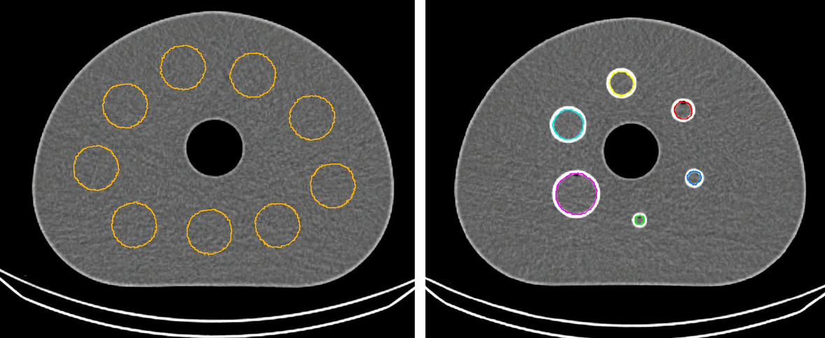
The left myocardium of the images was outlined with an approach similar to Germano [15]. Coefficient of variation (CoV = 100% × standard deviation/mean) of the segmented left myocardium counts was used as a measure of noise level for the different methods and acquisition times (Fig. 2). SSIM was calculated as

$$} = \frac \mu_ }}^ + \mu_^ }}\frac }}^ + \sigma_^ }},$$

(1)

where subscripts f and r refer to full time OSEM and reduced acquisition time OSEM or DL methods, μ is mean in the myocardium region, and σ is variance or covariance. SSIM measures the similarity between two images. The maximum value of SSIM is 1.0, which indicates that two images are identical. Paired t test was used to compare the statistical significance of the CoV and SSIM differences between DL methods and full/reduced acquisition time OSEM without denoising.

Outlined left myocardium. CoV of counts inside the outline was as a measure of noise. SSIM was also calculated using the outlined myocardium

TPD was calculated for each normal and defect study for each processing method (OSEM, CNN, RES, UNET and cGAN) at each noise level (full time, half time and quarter time) at stress and rest using QPS. TPD scores were used as observer rating for the presence of a perfusion defect. ROC curve analysis was performed based on the ratings and the knowledge of the presence of a defect. Area under the ROC curve (AUC) was used to measure perfusion defect detection performance. ROC curves and AUCs were calculated with MedCalc software (MedCalc Software Ltd, Ostend, Belgium). The statistical significance of the AUC differences between DL methods and full/reduced time OSEM without denoising was tested using the method presented by DeLong [16].