Study participantsCase-control studies of derivation stage EAS of the Chinese population

The subjects of four independent Chinese colorectal cancer GWAS (Additional file 1: Table S1 and Fig. S1) were recruited from the National ColoRectal Cancer Cohort (NCRCC), including NJCRC GWAS [1316 cases and 2207 controls [16], being part of the Genetics and Epidemiology of Colorectal Cancer Consortium (GECCO)], BJCRC GWAS (932 cases and 966 controls) [17], SHCRC GWAS (1116 cases and 1054 controls), and ZJCRC GWAS (1046 cases and 1184 controls). The detailed information is described in Additional file 1: Supplementary Materials.

EAS of the Japanese population

All participants of the Japanese GWAS were collected in the BioBank Japan Project (BBJ), and the population details have been published in a previous study [18]. We obtained the GWAS summary statistics of colorectal cancer (7062 cases and 195,745 controls) from the JENGER website.

EUR population (GECCO)

The GWAS datasets of GECCO consortia were deposited in the database of Genotypes and Phenotypes (dbGaP, phs001315.v1.p1; phs001415.v1.p1 and phs001078.v1.p1). All cases were confirmed by medical records, pathologic reports, cancer registries, or death certificates. The population details have been published in previous studies [5, 6]. After individual-level quality control (Additional file 1: Supplementary Materials), a total of 21,608 cases and 20,278 controls, which did not include datasets of Prostate, Lung, Colorectal, and Ovarian (PLCO) and Colorectal Cancer Study of Austria (CORSA), were retained for analysis.

EUR population (PLCO)

The PLCO cancer screening trial is a cohort study that aims to evaluate the accuracy and reliability of screening methods for prostate, lung, colorectal, and ovarian cancer [19], and the detailed information was described in our previous study [20]. We obtained the up-to-date GWAS summary statistics of colorectal cancer (2065 cases and 67,500 controls; October 18, 2022) in the EUR population from the PLCOjs website [21]. This study was approved by the ethics committees of the PLCO consortium providers (#PLCO-84).

Case-control studies of the validation stage EAS of the Chinese population

The confirmed cases from the JSCRC study were consecutively recruited from hospitals in Jiangsu province, China. The cancer-free control subjects were selected from individuals receiving routine physical examination at hospitals or those participating in community screening for non-communicable diseases in Jiangsu province. A total of 727 cases and 1452 controls were finally included in this study.

EUR population (CORSA)

The CORSA dataset included colorectal cancer and adenoma cases and colonoscopy-negative controls. Controls received a complete colonoscopy and were free of colorectal cancer or polyps [22]. We accessed the CORSA genotype data from dbGaP (phs001415.v1.p1) and kept 1289 cases and 1284 controls for subsequent analysis after the individual-level quality control process (Additional file 1: Supplementary Materials).

Longitudinal cohort of the testing stage

The UK Biobank cohort is a prospective, population-based study, which recruited 502,528 adults aged 40–69 years from the general population between April 2006 and December 2010 [23]. After individual-level quality control (Additional file 1: Supplementary Materials), a total of 355,543 participants were retained for our analysis (Additional file 1: Table S2) [24]. The follow-up time was calculated from baseline assessment to the first diagnosis of colorectal cancer [International Classification of Diseases, 10th revision (ICD-10) codes with C18-C20], loss to follow-up, and death or last follow-up (December 14, 2016). This study was conducted using the UK Biobank Resource under Application #45611.

GWAS meta-analysis of colorectal cancer

The genotyping, imputation, and SNP-level quality control procedures of all GWAS datasets are described in Additional file 1: Supplementary Materials. We used a multivariable logistic regression model to estimate the odds ratios (ORs) and 95% confidence intervals (CIs) for each SNP with the adjustment of sex, age, and principal components of ancestry, separately for each individual-level GWAS dataset.

We then performed a meta-analysis based on the summary statistics derived from EAS and EUR populations of derivation datasets (35,145 cases and 288,934 controls in total) using the inverse variance-weighted fixed-effects model, implemented by the METAL software [25]. After obtaining the summary statistics of the meta-analysis, we excluded SNPs if they (i) had substantial heterogeneity identified among studies (P value for heterogeneity test < 0.001) and (ii) did not pass filters in both EAS and EUR populations, a total of 4.7 million SNPs were retained for further analysis, and variants at P value < 5 × 10−8 were considered to be genome-wide significant. In the previously reported regions, genome-wide significant SNPs with Pconditional < 5 × 10−8 were considered as novel variants using conditional analysis with the Genome-wide Complex Trait Analysis (GCTA) software conditioning on the known SNPs [26].

Calculation of PRS

We calculated PRS to aggregate the weak effect of individual SNP [8], based on the following formula: \(\textrm=\sum_^n_i}_}\), where n means the number of SNPs, SNPi and βi are the number of risk alleles (i.e., 0, 1, 2), and weight carried by the ith SNP. The EAS-ancestry (Additional file 1: Table S3) and EUR-ancestry PRSs [10] were constructed using GWAS-reported variants. Furthermore, the development of candidate EAS-EUR PRSs was determined by five different approaches (Additional file 1: Supplementary Materials), including clumping and P value thresholding (i.e., C+T) approach (12 scores) [27], LDpred (11 scores) [28], lassosum (1 score) [29], LDpred2 (1 score) [30], and PRS-CSx methods (1 score) [31]. The 1000 Genomes EAS and EUR populations (Phase 3; 769 individuals) were used as a reference panel. The proportions of the different ethnic groups in the reference panel were consistent with those in the meta-analysis of EAS and EUR GWASs.

Calculation of lifestyle score

We calculated healthy lifestyle scores based on the eight lifestyle factors [32], including body mass index (BMI), tobacco smoking, alcohol consumption, waist-to-hip ratio (WHR), physical activity, sedentary time, red and processed meat intake, and vegetable and fruit intake (Additional file 1: Table S4). Each lifestyle factor was given a score of 0 or 1, with 1 representing the healthy behavior category, and the sum of the eight scores was used as the healthy lifestyle score. The detailed information is described in Additional file 1: Supplementary Materials.

Estimation of 5-year absolute risk

We estimated individual 5-year absolute risk for developing colorectal cancer by combining the relative risk (incorporating genetic risk and lifestyle) with the incidence rate of colorectal cancer and the mortality rate for all causes except for colorectal cancer [9], and the exact details of the calculations were described in our previous study [16].

Statistical analysis

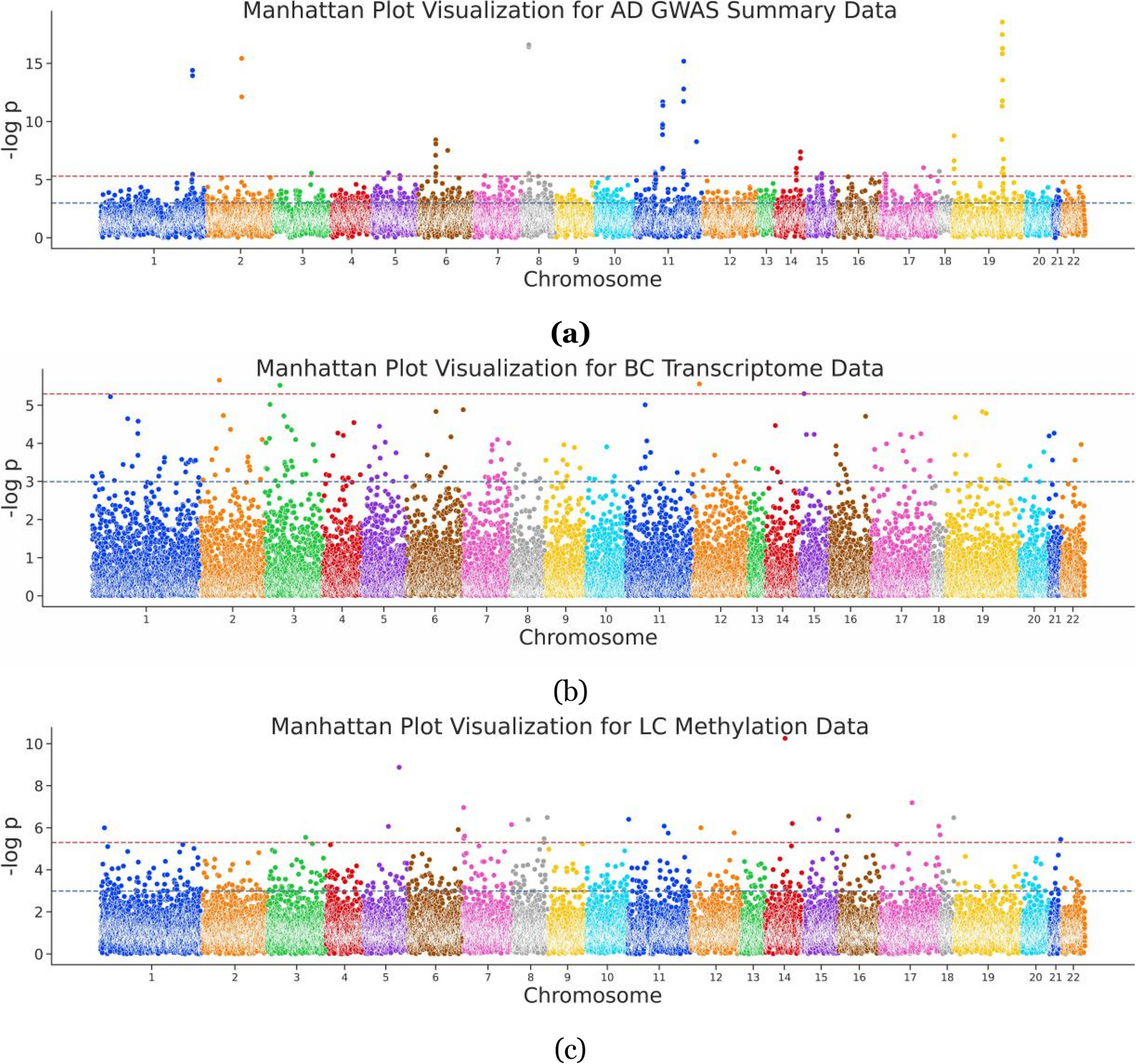
The population structure was estimated using the EIGENSOFT software [33], and the Manhattan plot and quantile-quantile plot based on the -log10 (P value) were created by using the R package qqman (https://cran.r-project.org/web/packages/qqman/index.html). We evaluated the discriminatory ability of PRSs derived from different approaches described above using the crude and covariates-adjusted area under the receiver operating characteristics curve (AUC) via the R package RISCA [34].

In the UK Biobank cohort, the Cox proportional hazards model was used to estimate the hazard ratios (HRs) and 95% CIs after adjusting for corresponding confounding factors. We compared the difference in the distribution of PRS between two or more groups by the Wilcoxon or Kruskal-Wallis tests. Participants were classified into ten equal subgroups according to the decile distribution of PRS and categorized into low (bottom 10%), intermediate (10–90%), and high genetic risk (top 10%) subgroups for group comparisons. Similarly, participants were classified into unfavorable (0 and 1 score), intermediate (2 and 3 score), and favorable (≥ 4 score) lifestyle subgroups based on lifestyle scores ranging from 0 to 8. The log-rank test was used to evaluate the difference in cumulative incidence (one minus the Kaplan-Meier estimate) stratified by different levels of PRS or lifestyle scores. The incidence proportion and 95% CI in each group were estimated by the exact Poisson test. The R package Shiny (https://cran.r-project.org/web/packages/shiny/) was used to construct the colorectal cancer risk prediction web server, which was freely available and open source.

In addition, to assess the robustness of the results, we performed the following sensitivity analyses: (i) excluded incident colorectal cancer cases that had occurred during the first year of follow-up; (ii) evaluated the associations using ancestry-corrected PRS: briefly, fit a linear regression model using the first ten principal components of ancestry to predict PRS, and the residual from this model was used to create ancestry-corrected PRS; (iii) healthy lifestyle categories were reclassified to unfavorable (0, 1, and 2 score), intermediate (3 and 4 score), and favorable (≥ 5 score) lifestyle groups; and (iv) excluded non-colorectal cancer participants with other cancers that occurred during the time of follow-up.

All other statistical analyses were performed using the R software (version 3.6.1, https://cran.r-project.org/), and a two-sided P value less than 0.05 was considered as significant.