Phantom preparation

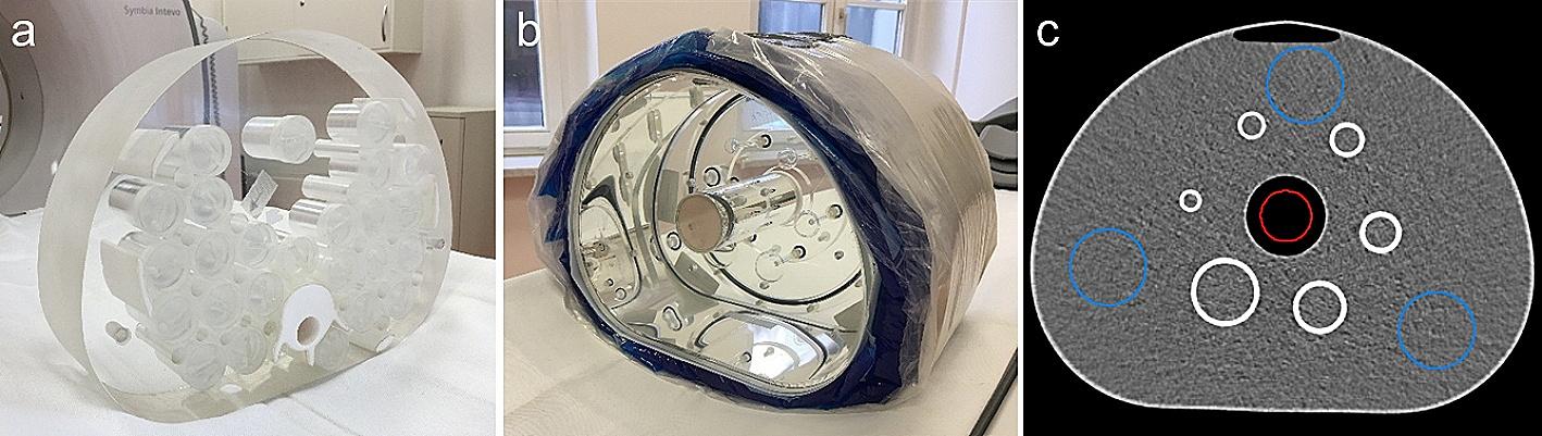
Several phantoms were used in this study. A PET cylindrical flood phantom and a NEMA image quality (IQ) body phantom (Model PET/IEC-BODY/P) were used for calibration and validation purposes, while the anthropomorphic Torso (ECT/TOR/P, (Data Spectrum, Hillsborough, NC)) and LK-S Kyoto Liver/Kidney phantoms were used for validation and quantification accuracy estimation (Fig. 1).

Fig. 1

a NEMA IQ phantom and b PET cylindrical flood phantom used for calibration. Anthropomorphic c Torso (ECT/TOR/P, (Data Spectrum, Hillsborough, NC)) and d LK-S Kyoto Liver/Kidney phantoms used for 177Lu activity quantification validation in spheres and large organs

The PET cylindrical flood phantom was filled with an activity of 1.4 GBq of 177Lu-DOTATATE leading to an activity concentration of 0.25 MBq/mL. This phantom was used to calculate a CF from a uniform activity distribution [14] following the conventional method. The NEMA IQ phantom was used for both calibration and validation. This phantom contains six fillable spheres with volumes of 26.52 cc, 11.49 cc, 5.71 cc, 2.84 cc, 1.23 cc and 0.44 cc and a background compartment of 9.7 Liter. This phantom was first used to determine CFs for different sphere volumes according to the conventional method (NEMA Cal. 1 acquisition). The spheres contained a uniform 177Lu-DOTATATE activity concentration of 2.62 ± 0.04 MBq/cc, while the background has a concentration activity of 0.16 MBq/cc. Secondly, the NEMA IQ phantom was prepared with varying surrounding background activity to assess the effect of the background activity (NEMA Cal. 2 acquisition). The six spheres were filled with a uniform 177Lu-DOTATATE activity concentration of 1.89 ± 0.04 MBq/cc, and the phantom was scanned with five different background activity concentrations (0, 0.11, 0.14, 0.19 and 0.31 MBq/cc). CFs were calculated for all the different configurations. One additional NEMA IQ phantom was prepared for validation purpose with spheres activity concentration of 2.14 ± 0.01 MBq/cc and a background activity concentration of 0.14 MBq/cc (NEMA Val. acquisition).

The anthropomorphic Torso Phantom (Torso Val. phantom) simulates the upper torso of average subjects and was used for quantification accuracy validation. The phantom includes left and right lungs filled with polystyrene and water to simulate lung tissue density, a 1.2-L liver fillable compartment, a background region and spine. The 26.52 cc and 5.71 cc NEMA IQ spheres filled with 177Lu-DOTATATE activity concentration of 2.66 MBq/cc were inserted in the 0.26 MBq/cc liver and 0.03 MBq/cc background regions, respectively. The anthropomorphic LK-S Kyoto Liver/Kidney phantom (Liver/Kidney Val. Phantom) was used to assess the quantification accuracy for large organs, i.e., liver and kidneys, and for lesions. The phantom was prepared by inserting the 26.52 cc, 11.49 cc and 5.71 cc NEMA IQ spheres with a respective 177Lu-DOTATATE activity concentration of 6.14 MBq/cc, 4.77 MBq/cc and 3.56 MBq/cc in different regions of the anthropomorphic phantom. The 26.52 cc and 5.71 cc spheres were inserted in the 0.27 MBq/cc liver compartment, and the 11.49 cc sphere was inserted in the 0.08 MBq/cc background compartment. The left and right kidneys contained a 177Lu activity concentration of 0.63 MBq/cc and 0.89 MBq/cc, respectively. Table 1 summarizes the 177Lu activity concentrations contained in the different phantoms and spheres.

Table 1 Phantom acquisitions and configurationsImage acquisition and reconstruction

All phantom acquisitions were performed using a Discovery NM/CT 670 (International General Electric, General Electric Medical Systems, Haifa, Israel) gamma camera. This system combines a dual-head coincidence SPECT camera with an axial field of view (FOV) of 40 × 54 cm, a 9.5-mm-thick NaI(Tl) crystal, and 59 photomultiplier tubes (PMT). All SPECT images were acquired with a 20% energy window around the main photopeak of 177Lu (208 keV; 11% probability) with medium-energy general purpose (MEGP) collimators. The different acquisitions were performed by applying 60 views over 360° (30 angular steps per head, 6° angle step) with a 30-s exposure per frame (15 min acquisition) in a 128 × 128 matrix size (4.4 mm pixels). In addition, for the NEMA Val., Torso Val. and Liver/Kidney Val. phantoms, 20-s and 10-s per frame acquisitions were obtained.

Image reconstruction was performed using the General Electric (GE) Dosimetry toolkit (DTK) software [19] available for the Xeleris 3.0 Workstation (International General Electric, General Electric Medical Systems, Haifa, Israel). The ordered subsets expectation maximization (OSEM) algorithm with a subset and iteration product of 100 (10 iteration and 10 subsets) was used in order to obtain counts convergence in small VOIs [12]. Additionally, attenuation correction (from CT attenuation maps) and resolution recovery (for reducing image blurring) included in the Xeleris 3.0 workstation were used. For scatter correction, the dual energy window (DEW) method was used. This method consists of measuring the scatter in an energy window juxtaposed just below the main photopeak window (208 keV) that was placed ± 10% around 166.4 keV [20]. Then, a pixel-by-pixel correction subtracting the scatter counts from the main photopeak counts was performed. This correction uses a weighting factor, which depends on the width of the main peak and scatter energy windows [6].

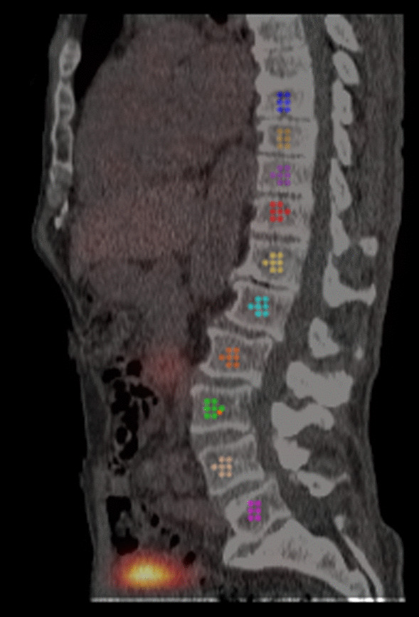
Image analysis

Processing in GE DTK includes either semi-automatic (threshold approach) or manual three-dimensional delineation of the VOIs on SPECT or CT images. For the PET cylindrical phantom, the semi-automatic delineation tool was used on the SPECT image to delineate the whole phantom activity. For determination of background CF in the NEMA Cal. 2 acquisition, six rectangular VOIs were drawn manually across the whole length of the phantoms background. The sphere VOIs in the different phantoms (NEMA IQ, Torso Val. and Liver/Kidney Val.) were drawn manually on CT images using the DTK sphere tool. For liver and kidneys in the anthropomorphic phantoms, VOIs were drawn manually on CT images and were placed over the whole organs. It is noteworthy that the GE DTK software does not allow copying the VOIs delineated on a SPECT/CT acquisition to another study. Therefore, all sphere VOIs were drawn again on attenuation SPECT images for each acquisition (by the same user). Figure 2 shows an example of the drawn sphere and background VOIs using the GE DTK software. Finally, as output, the GE DTK software gives the volume of the VOIs, the total number of counts and the number of counts per voxel in the drawn VOIs.

Fig. 2

a, b Spheres and c, d background volumes of interest (VOIs) drawn on the NEMA IQ Cal. phantom using the General Electric Dosimetry toolkit (GE DTK) software

Calibration factors calculation

The CFs [cps/MBq] for both methods were calculated using the following formula:

$$} = \frac}_}}} }}}}} *V_}}} *C_}}} }}$$

(1)

where \(}_}}}\) is the total counts in the delineated VOI, \(V_}}}\) is volume [cc] of the VOI, \(C_}}}\) is the calibrated activity concentration [MBq/cc] in the VOI region, and \(T_}}}\) is total image acquisition time in sec (product of the time per view and number of views).

Calibration factors—conventional method

Background/Organ calibration factors The background CF for the conventional method is used to quantify large organs (kidneys and liver) and was calculated from the PET cylinder acquisition by delineating the whole phantom volume and using Eq. 1.

Sphere/lesions calibration factors CFs for the three largest spheres of the NEMA Cal. 1 acquisition were calculated using Eq. 1.

Calibration factors—SBVR method

Background calibration factors The background CF for the SBVR method was calculated using an alternative method with the aim to simplify the entire calibration process by using a single phantom (i.e., NEMA IQ). The background CF was obtained from each of the four NEMA Cal. 2 acquisitions with hot background by averaging the CFs obtained in the six rectangular VOIs as described above. In total, four background CFs were obtained from the NEMA Cal. 2 across the five acquisitions. (Background CF was not calculated for the NEMA Cal. 2 acquisition with cold background.) The four background CFs were averaged and the resulting background CF obtained with the SBVR method was compared to the conventional background CF.

Sphere/lesions calibration factors The CFs for the three largest spheres of the NEMA Cal. 2 acquisition (26.52, 11.49 and 5.71 cc) were determined from the five acquisitions from cold to hot background (range 0–0.31 MBq/cc) using Eq. 1, as described before (Table 1). In total, 15 CFs were calculated for the five different NEMA Cal. 2 acquisitions.

For a given sphere, the CFs varied in the different acquisitions as the function of the background concentration activity. Therefore, CFs were expressed as function of the sphere-to-background activity concentration ratio (SBAR of ∞:1, 17:1, 14:1 10:1 and 6:1, respectively, to the 0, 0.11, 0.14, 0.19 and 0.31 MBq/cc background), as well as the sphere volume. In addition, the CFs were expressed as function of sphere-to-background voxel ratio (SBVR) as well as the sphere VOI volume.

Sphere-to-Background Voxel Ratio (SBVR) Sphere-to-background voxel ratio (SBVR) was defined as the ratio between the total counts per voxel in a VOI and the total counts per voxel in a surrounding background VOI, as:

$$} = \frac}_}}} }}}_}}} }}$$

(2)

Here, \(}_}}}\) is the total counts per voxel in a VOI and \(}_}}}\) is the total counts per voxel in the background VOI. The SBVR was calculated for each of the three largest spheres and for every NEMA Cal. 2 acquisition. The total counts per voxel in the background were calculated by averaging the total counts per voxel in each of the six rectangle VOIs in each acquisition. In total, 12 SBVRs were calculated for the three largest spheres across the four NEMA Cal. 2 acquisitions with hot background. In order to assess the effects of the background on CFs for all background activity concentrations, CFs were plotted against SBVR as a linear function for each of the three spheres separately. For cold background, the spheres SBVR values could not be calculated directly using Eq. (2) due to the absence of activity in the background (SBVR values of infinity). Instead, the SBVR value leading to a maximum CF for each sphere was obtained by determining the point of intersection between the CF versus SBVR linear curve and the cold background CF value for each of the three spheres.

To obtain the CF versus SBVR calibration curves for a larger series of volumes, the CFs were expressed as function of the VOI volume by exponentially fitting the CFs obtained for the three spheres (from the linear functions) and for a fourth large VOI. The latter was calculated for different SBVR values using a transition factor (TF) calculated from cold background. TF was calculated by dividing a background CF value - CFBG, where the PVE is negligible and there are no background effects, by the CF of the largest sphere in the cold background acquisition - \(CF_}} \right)}}\) as follows:

$$} = \frac}_}}} }}}_}} \right)}} }}$$

(3)

Therefore assuming that TF stays constant for all background activity concentrations, a large volume CF for a given SBVR is obtained by multiplying the corresponding CF26.52 by TF. Combining both CF versus SBVR and CF versus VOI volume curves resulted in the mapping of the CFs as function of SBVR and the VOI (lesion) volume.

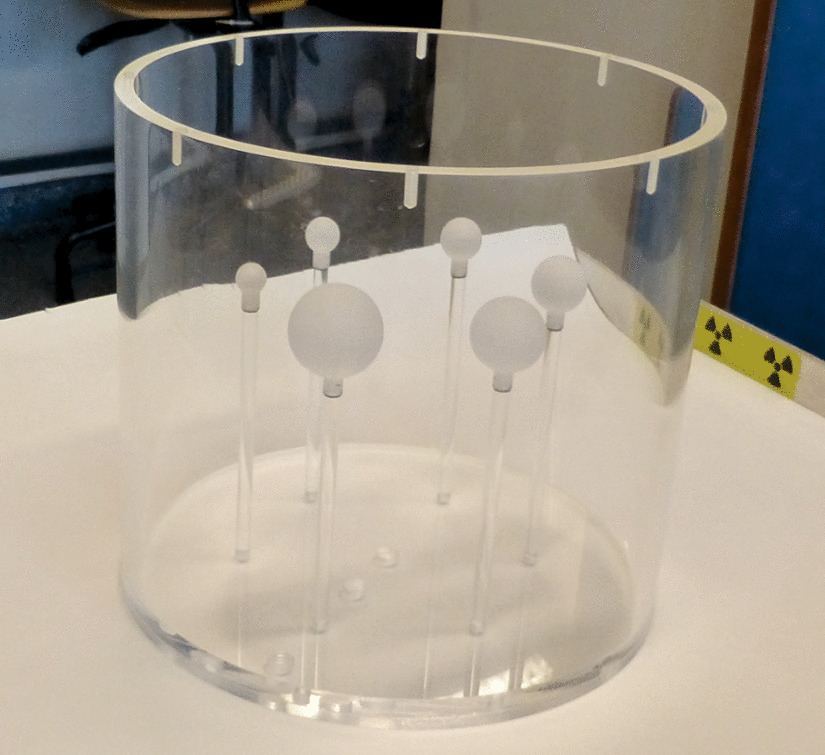
Validation of quantitative imaging

Validation of the conventional and SBVR calibration methods was performed using the NEMA Val., Torso Val. and Liver/Kidney Val. acquisitions. The conventional quantification method [12, 21] uses the sphere CFs calculated from NEMA Cal. 1 acquisition and the background CF calculated from PET cylindrical phantom for quantification of the large organs, without taking background effects into consideration. For the SBVR method, quantification was done using the CF map. The SBVR and VOI volume values were obtained from delineation of the spheres, liver, and kidneys and their surrounding background in the anthropomorphic and NEMA IQ (NEMA Val. acquisition) phantom acquisitions. Both values (VOI volume and SBVR) were then plugged into the CF map to obtain a corresponding CF which is used for quantification. Moreover, SBVR values were calculated using different background delineation methods due to the non-uniformity of the background around the spheres and around the large organs (liver and kidneys). For example, Fig. 3 shows different configurations where spheres are close to two different background regions. Indeed, Fig. 3b shows that the large sphere (green) is surrounded by both the liver activity and the phantom background activity. For the small sphere (blue), the effects of the surrounding activities on the quantification may be even more important since the latter is surrounded by phantom background activity on one hand and by air (null activity) on the other hand. To address this problem, three delineation methods (Fig. 3a–c) were tested. In the first method (Fig. 3a), a thick background ring was placed around the sphere VOI. The second method (Fig. 3b) includes an additional thin separation ring placed between the sphere VOI and the background ring to eliminate spillover from the sphere VOI to the background. In the third method (Fig. 3c), random background spherical VOIs were placed around the sphere VOI and the counts per voxel were calculated as the average across the background spherical VOIs. Validation was also performed for the different time-per-view settings for the NEMA Val., Torso Val. and Liver/Kidney Val acquisitions.

Fig. 3

Delineation methods for anthropomorphic phantoms. In methods a 1 and b 2, the inner VOI (green or blue) represents the sphere VOI, while the outer thick ring delineates the surrounding background VOI. In method 2 (b), the thin middle ring is used to separate both VOIs to prevent spill in/out from sphere to background. With method 3 (c), random background spherical VOIs are placed around the sphere VOI

Statistical analysis

The CF versus SBVR curves were fitted using a linear fit. The CF versus VOI volumes were fit using an exponential fit. The best fit has been found to be with the following structure:

$$f\left( x \right) = Ae^ + Ce^$$

CFs linear and exponential fitting was performed using MATLAB (MATLAB Release 2022a, The MathWorks, Inc., Natick, MA, USA).

Comparison between the conventional, SBAR and SBVR methods was assessed by comparing the quantification accuracy of the different methods as the relative difference between the true injected activity concentration in the spheres/organs and the estimated activity concentrations using the different calibration methods.