INTRODUCTION

Accidental inhalation of plutonium at the workplace is a non-negligible risk, even when rigorous safety standards are in place. Over the past 80 y, Los Alamos National Laboratory (LANL) has manufactured plutonium for different purposes; for example, the production of nuclear batteries, such as Multi-Mission Radioisotope Thermoelectric Generator (MMRTG) to support the US national interest in space exploration (LANL 2012). An MMRTG converts the heat generated by the radioactive decay of 238Pu into electricity, which generates dependable electrical power that is used by spacecraft to explore remote locations, such as the frigid surface of Mars. It is also well known that nuclear emergencies may result in radionuclide intakes.

The intake and retention of plutonium in the human body may be a source of concern, as plutonium is known to be an undesirable material to be taken into the human body. If there is a suspicion of a significant intake of plutonium (i.e., 20 mSv committed effective dose) (Gerber and Thomas 1992), medical countermeasures such as chelation treatment may be offered to the worker. Chelation treatment involves the administration of chelating agents to remove heavy metals (e.g., plutonium) from the body as an attempt to reduce the internal radiation dose. In 2004, the US Food and Drug Administration (US FDA) approved two chelating agents, commonly known as Ca-DTPA and Zn-DTPA (trisodium calcium/zinc salts of diethylenetriaminepentaacetic acid), to treat significant intakes of plutonium, americium, or curium as part of its ongoing effort to protect the public from terrorist attacks and nuclear accidents (US FDA 2004; Hameln Pharmaceuticals 2013a and 2013b).

However, the administration of chelating agents such as Ca-DTPA affects plutonium’s normal biokinetics inside the body. In particular, chelation treatment enhances plutonium’s rate of excretion. Consequently, the standard biokinetic models for plutonium cannot be used to model the bioassay data affected by chelation (i.e., the bioassay data collected when chelation treatment was ongoing and sometime after the treatment ended) to estimate the intake and assess the internal radiation dose (NCRP 1980; IAEA 1996; ICRP 2015). A recent review of the literature compiled the available methods for analysis of bioassay data affected by chelation treatment (Dumit et al. 2020a). However, there is currently no consensus chelation model available, even after 50+ years of research (Breustedt et al. 2012; Dumit et al. 2020a).

The present work aimed to interpret the bioassay data of a worker involved in an inhalation incident and treated with Ca-DTPA due to a glovebox breach at LANL’s plutonium facility. The objectives of this work are to describe the incident, model the chelation-affected and non-affected bioassay data, estimate the plutonium intake, and calculate the internal radiation dose. Hence, a new chelation model (Dumit et al. 2020b) was used in this study.

MATERIALS AND METHODS Case description

The inhalation incident, along with a full description of the health physics response, has been described in-depth by Poudel et al. (2023). Briefly, the incident consisted of a glovebox breach at LANL’s plutonium facility involving 15 radiation workers. However, this study focuses on examining the data of only one of the affected individuals—the only one who received chelation treatment, referred to hereafter as the “worker.”

After finishing up work handling 238PuO2 material, the glovebox worker removed his hands from the gloves and, while tying up the gloves together (outside the glovebox, to secure them), the alarm of a portable continuous area monitor (CAM) in the room rang. The worker immediately exited the room, and while he was walking to the adjacent corridor, additional CAMs alarmed. As usual, the worker was wearing appropriate personal protective equipment (PPE), including safety glasses, anti-contamination (anti-C) coveralls and gloves, shoe covers, and a COVID-19 face mask (due to the novel coronavirus pandemic and the use of face masks required by LANL policies).

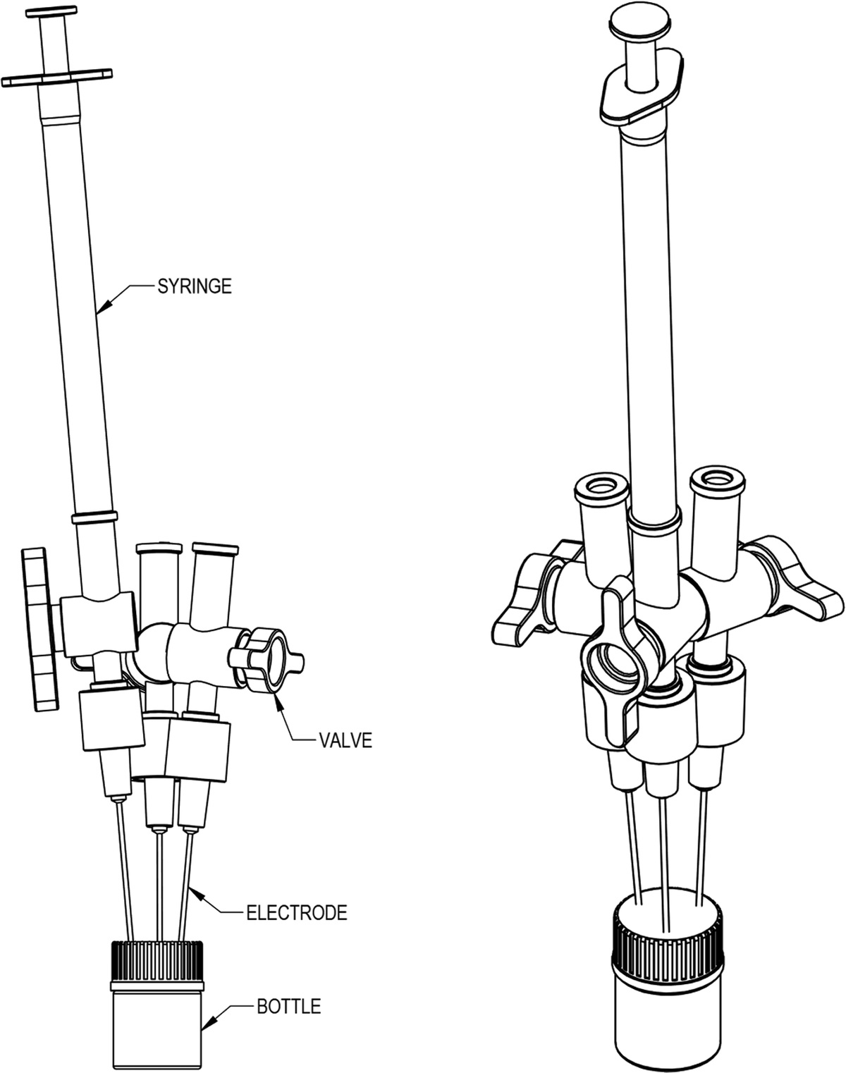
The worker went to the decontamination room and was cleaned with soap, water, and decontamination wipes until all hair and skin contamination levels were non-detectable. Nasal swabs were obtained from the worker, with a total activity (sum of both sides) of 764 dpm. The worker was issued “prompt action” bioassay kits, which consist of a series of successive samples collection. On the same day as the incident, the worker went to LANL’s Occupational Medicine and received chelation treatment with Ca-DTPA.

Bioassay data

The worker’s bioassay data used in this study are summarized in Table 1, along with the normalization uncertainties (primarily because of biological variabilities) used. A total of 48 data points (nData) were used.

Table 1 - Bioassay data used. Bioassay data Affected by chelation?a Number of data (nData) Additional informationb Normalization uncertainties Sc SFd Urine 72 hours Yes 1 Based on 3 ‘true 24-hour’ collections 0.3 1.3 Urine 24 hours Yes 25 All ‘true 24-hour’ collections 0.3 1.3 Urine 24 hours No 20 17 ‘true 24-hour’ collection, and
3 ‘simulated 24-hour’ collection 0.3 1.3 Feces 72 hours Yes 1 Combination of all of the samples collected over three days 2.5 12.2 Nasal swabse No 1 Sum of both sides 2.1 8.2 48 Total nData

aAffected by chelation means the bioassay was collected either when treatment was ongoing or during the 100-day period after the last chelation injection. Not affected by chelation means the bioassay was collected after the 100-day period after the last chelation injection.

bA ‘true 24-hour’ bioassay collection means that all urine voids were collected during the 24-hour period. A ‘simulated 24-hour collection’ involves collecting four samples: 1) evening voiding of the first day, 2) next morning’s first voiding, 3) evening voiding of the second day, and 4) next morning’s first voiding, normalized using volume and excess specific gravity.

c,dScattering factor (SF) = geometric standard deviation (GSD) = exp(S). The Results Section shows the plots with error bars, which reflect the values of S used (and help to visualize them).

eNasal swab results were used for the purpose of estimating the intake (Miller et al. 2023a).

The measurements of the first three urine collections were summed up over a 72-h period, and the fecal data was collected as a 72-h sample. For the urine samples, the data aggregation was used to lessen dependence on timing of sample collection, which is poorly known experimentally and theoretically. For the fecal samples, they were analyzed as a 72-h collection (i.e., a combination of all of the feces the individual produced over 3 d). It must be noted that early fecal sampling was not possible because LANL currently does not have the in-house capability to analyze fecal samples—fecal sample analysis is conducted by an outside laboratory. Thus, there is only one fecal sample (see Table 1), which was collected around day 50 (after the intake).

Measurement uncertainties were estimated as described elsewhere (Dumit et al. 2020b). Briefly, the likelihood function was assumed to consist of measurement uncertainty convoluted with normalization uncertainty. Measurement uncertainty was either exact Poisson using count quantities or normal with normal “measurement” uncertainty, either as reported or assumed to be small. The normalization uncertainty was assumed to be lognormal, characterized by a lognormal standard deviation S that was estimated [scattering factor = geometric standard deviation (GSD) = exp(S)]. The assignment of normalization uncertainty was done on a dataset/type of measurement basis, where the largest reasonable value of S in our estimation was used for normalization uncertainties for different types of measurements (as shown in Table 1).

Chelation treatment

Upon discussions with medical staff, an internal dosimetrist, and Radiation Emergency Assistance Center/Training Site (REAC/TS) staff, the worker agreed to receive chelation treatment. The worker was given the first administration of Ca-DTPA (1 gram) intravenously on the day of the incident and the second Ca-DTPA injection (also 1 gram) on the next day. The worker provided bioassay samples during the 2 d of chelation treatment and afterward.

Software

The software package IDode (Miller et al. 2012, 2019) was used in this study for all calculations performed. IDode is able to handle second-order kinetics, which are important for chelation modeling, and is able to calculate parameter uncertainties using Markov Chain Monte Carlo (MCMC). The software package Activity and Internal Dose Estimates (AIDE) (Bertelli et al. 2008) was used in this work for benchmarking the biokinetic models implemented in IDode, when possible, and also for validation of IDode’s dosimetric models (in the context of plutonium inhalation).

It must be noted that IDode is a radiation dose-calculation software and is designed to work with units of activity of the radionuclides involved. As explained by Dumit et al. (2020b), the software does allow the use of arbitrary units for non-radioactive materials. The units used in this study were becquerel (Bq) for plutonium and gram (g) for Ca-DTPA (the non-radioactive material). IDode also allows the user to use different calculation modes, such as forward model predictions, fit, and MCMC.

Biokinetic and dosimetric models

The biokinetic models used in the present study are listed in Table 2. All models were constructed in IDode software (Miller et al. 2012, 2019).

Table 2 - Biokinetic and dosimetric models used. Model type Referencea Model identification Varied parameters during fit Biokinetic ICRP 1979 ICRP 30 Gastrointestinal (GI) tract model None (all fixed)b Biokinetic ICRP 1994 ICRP 66 Inhalation model Intake, solubility parameters, and AMADc Biokinetic Leggett et al. 2005 Plutonium systemic model None (all fixed)b Biokinetic Dumit et al. 2020b Chelation model None (all fixed)b,d Dosimetric ICRP 1991 ICRP 60 dosimetric system —

aICRP = International Commission on Radiological Protection.

bNone (all fixed) = the default parameter values published in the original publications were used, i.e., not allowed to vary during the fitting.

cFor more details, please, refer to Table 3. (AMAD = Activity Median Aerodynamic Diameter).

dThe Ca-DTPA amounts and times were specified according to the treatment protocol administered to the worker.

Regarding the biokinetic models, the inhalation model published in ICRP Publication 66 (ICRP 1994) was linked to the ICRP Publication 30 Gastrointestinal (GI) tract model (1979) and the plutonium systemic model (Leggett et al. 2005), which was linked to the chelation model (Dumit et al. 2020b). Regarding the dosimetric models, the default ICRP Publication 60 (ICRP 1991) dosimetric system was used, including the tissue weighting factors. The dosimetry also included ICRP Publication 107 (ICRP 2008) nuclear decay data and absorbed fraction data (i.e., alpha absorbed fractions), as detailed by Cristy and Eckerman (1993).

Chelation modeling approach

Differently from the “standard modeling approach” to dose assessment (which consists of only using bioassay data non-affected by chelation treatment), this study uses a “chelation modeling approach” as described elsewhere (Breustedt et al. 2009, 2010; Dumit et al. 2019a, 2019b, 2020b). Briefly, model structures describing the biokinetics of the free chelating agent (DTPA) and the Pu-DTPA chelate are linked and combined to the plutonium systemic model via second-order kinetics to describe the transfer of material and the in vivo chelation process. All data are included, the chelation-affected bioassay data (i.e., the bioassay data collected during treatment and until 100 d after the chelation treatment ended), and the non-affected bioassay data (the bioassay data collected after the effect of chelation treatment has ceased).

Maximum likelihood and MCMC methods

In this study, the maximum likelihood method (alternately minimum χ2) was implemented, as described in detail by Miller et al. (2002) and Poudel et al. (2018, 2023), to calculate the model parameters given the model structure and the bioassay data.

Briefly, the likelihood function used is described below. The purpose of the likelihood function is to calculate the probability of observing Mi (measurement value) given the true value of I, representing intake and other model parameters:

LiI=PMiI.

Having independent measurements, n, the likelihood functions for the individual measurements result in the combined likelihood function below:

LI=∏i=1nLiI.

Hence, an error function proportional to the negative log of the likelihood can be defined:

χifiI≡±−2lnLiI,

where χi (fi(I)) is the deviation of the forward model prediction, which is a function of the forward-model-calculated value corresponding to the measurement, for the ith measurement. The combined likelihood function can then be written as L(I) = exp(−χ2/2) with:

χ2=∑i=1nχifiI2.

The maximum likelihood method thus consists of minimizing the sum of χi2 (hereafter, χ2).

In this work, the likelihood functions for the datasets used (Table 1) were assumed to be exact-Poisson/lognormal for urine data and normal/lognormal for fecal and nasal swab data (Miller 2008; Poudel et al. 2018; Miller et al. 2023a). A lognormal normalization/calibration uncertainty S, corresponding to a scattering factor exp(S), was included as shown in Table 1.

The MCMC method used in this study has been described elsewhere (Miller 2017). Briefly, the MCMC method yields a chain of model parameter values, which constitute a sample from the posterior distribution. The chain is used to calculate the posterior distribution of any function of the parameters (e.g., doses). The dose assessment results were obtained from MCMC and are reported as posterior average and standard deviation (SD).

Statistical analysis

Minimization of χ2 was performed using the “fit” calculation mode in IDode software, where, starting from some given point in parameter space, the unknown parameters are varied in order to find a minimum χ2 point.

To evaluate the data fitting for a linear model, the minimum value of χ2 divided by the number of degrees of freedom (number of data minus number of parameters) should be approximately 1. Miller (2017) points out that for a linear model, the chain-average of χ2/nData is approximately 1 regardless of the number of degrees of freedom. The data normalization uncertainties are not precisely known, and adjusting them has a pronounced effect on χ2 and also affects the parameter uncertainties calculated using MCMC. If the model does not fit the data, the parameter uncertainties calculated using MCMC would not be meaningful. On this basis, for linear or nonlinear models such as the one considered here, to have meaningful calculated parameter uncertainties, the chain-average χ2/nData should be approximately 1 (self-consistency of model with data).

RESULTS AND DISCUSSION Implementation of biokinetic and dosimetric models

The biokinetic models used in the present study (Table 2) were constructed in IDode software (Miller et al. 2012, 2019). Most of the biokinetic models implemented in IDode were benchmarked against the AIDE software package (Bertelli et al. 2008), except for the chelation model, due to the fact AIDE currently does not calculate second-order kinetics. IDode’s dosimetric system implementation in the context of plutonium inhalation dosimetry was also validated against the AIDE software. Benchmarking results of urine and fecal excretions, blood, alveolar interstitial, and extra thoracic lymph nodes were successfully validated with minimal deviation (less than 1% difference between both software packages).

The inhalation model used two intake components, both of which were described using the ICRP formalism shown in Fig. 1a. Different model structures were tried, and the transfer rates were optimized until a satisfactory fit was obtained. The final rates are shown in Table 3.

Fig. 1: An inhalation intake results in deposition in various regions of the lung: (a) Illustration re-drawn from ICRP Publication 66 (1994) showing the compartment model for time-dependent absorption into the blood. Reprinted with permission of the ICRP, www.icrp.org; (b) Solubility model and parameters representing the first intake component (“up-down”), built as “compartments-in-series,” which had joint values of transfer rates to their absorption into blood. Table 3 - Fitting results of the intake amounts and transfer rate values for the solubility parameters and AMAD. 1 st Intake Component (“up-down”) Parameter Transfer rate (d-1) Values Varied or fixed?a,b Intake - 188.9 Bq Varied Sp 0 - Fixed Spt 9.7 × 10-2 - Jointly variedc St 9.7 × 10-2 - Jointly variedc Sb 9.7 × 10-2 - Jointly variedc fb 1 - Fixed AMAD - 2.01 μm Jointly variedd f 1 (GI Tract absorption) 1 × 10-4 - Fixed 2 nd Intake Component (soluble and insoluble) Parameter Transfer rate (d-1) Values Varied or fixed?a,b Intake - 7.5 Bq Varied Sp 82.1 - Varied Spt 3.5 - Varied St 0 - Fixed Sb 0 - Fixed fb 0 - Fixed AMAD - 2.01 μm Jointly variedd f 1 (GI Tract absorption) 0 - Fixed

aThe last column asks “varied or fixed?” referring to whether the transfer rates were allowed to vary during the fit operation, or if they were set as a fixed value (unchanged during and after fitting).

bA total of 6 parameters were allowed to vary during the fitting. Please, note that the “jointly varied” parameters count as one parameter, since they are shared.

cJointly varied = varied as joint (or shared) parameter with each other, i.e., set to have equal values (represented by the Sud parameter in Fig. 1b).

dJointly varied = the AMAD values were varied as joint (or shared) parameters with each other in relation to the intake, i.e., set to have equal values.

The first intake component (“up-down”) was parameterized by the solubility parameters Spt = St = Sb, and was built as three compartments in series with equal transport, Sud, “ud” standing for “up-down” (Fig. 1b). One can easily verify by induction that for n compartments in series with equal transport rate s and the first compartment having initial value 1 at t = 0, the rate of transfer out of the last compartment is given by s(st)(n − 1) e−st so for n > 1 has an “up-down” character.

The second intake component can be thought of as being comprised of two simple intakes, soluble and insoluble. The ICRP solubility model structure shown in Fig. 1a is equivalent in this case to the two simple intakes: a fraction of deposition Sp/(Sp + Spt) with dissolution rate Sp + Spt (soluble), and a fraction Spt/(Sp + Spt) with dissolution rate 0 (completely insoluble).

Solubility of the 238Pu material

An in-depth investigation of the material solubility involved in the incident using material from a fixed head air sampler located above where the worker was working was conducted by LaMont et al. (2022) with an alternate data analysis by Miller et al. (2023b). LaMont et al. (2022) state that the material was 99% insoluble and 1% soluble. Miller et al. (2023b) also state that the material was 99% insoluble and 1% soluble but with the finding that the soluble component was actually composed of three distinct behaviors, including a small ‘up-down’ component similar to what is seen here—a typical behavior observed with ‘ceramic’ 238Pu material at LANL attributed to increased solubility as the material matrix breaks down because of alpha recoil (Diel and Mewhinney 1980; Fleischer and Raabe 1978; Hickman et al. 1995; Poudel et al. 2019).

This study does not use either the results from LaMont et al. (2022) or Miller et al. (2023b), because the worker was wearing a COVID-19 mask, which by selectively filtering out larger particles, potentially biased the solubility characteristics of the inhaled aerosol. The nasal swab activity (764 dpm or 12.7 Bq) was a very small fraction of the contamination on the COVID-19 mask (5 × 105 dpm or 8,300 Bq). Hence, it is likely that the inhaled aerosol material was not the same as the aerosol that was measured (from the air filters) in the LaMont et al. (2022) solubility study.

Modeling of bioassay data

The model is compared against the bioassay data in Figs. 2 through 4 (urine, feces, and intake from nasal swabs, respectively). A χ2/nData of 0.98 for the entire dataset, 48 nData, was obtained during a simultaneous 6-parameter fit (Table 3). All other model parameters were fixed, as stated in Table 2. This result indicates that the biokinetic models used (Table 2) successfully represent the combined bioassay data (Table 1).

Fig. 2:

Fit to the combined 238Pu data in urine. Legends on the plot: black diamond = urine 72-h data point, affected by chelation treatment; black ellipses = daily urine, affected by chelation treatment; black triangles = daily urine, 100 days after the last chelation injection (i.e., non-affected by chelation treatment).

Fig. 3:

Fit to the 238Pu data in feces. Legend on the plot: black ellipse = feces 72 h, affected by chelation treatment.

Fig. 4:

Fit of the nasal swab results as an estimate of the 238Pu intake. Legend on the plot: NS = nasal swab; Black ellipse = intake calculated from the nasal swab data.

The plots (Figs. 2 through 4) show the error bars, which reflect the values of S used (and help to visualize them). The interested reader is also referred to Table 1, where the scattering factor [SF = exp(S)] values are also presented for comparison with literature values (Castellani et al. 2013; European Commission 2018). The normalization uncertainties for the urine data are in agreement with published SF values, whereas the fecal data uncertainties are in disagreement (Castellani et al. 2013; European Commission 2018). It must be noted that the SF values for 72-h fecal samples from the literature (Castellani et al. 2013; European Commission 2018) were calculated from the SF values for 24-h fecal samples. As shown in Table 1, this study uses 72-h fecal sample.

As explained by Poudel et al. (2023), there were various challenges in modeling this dataset, including the fact that the solubility of the material was not well known initially, the biokinetics of 238Pu oxide forms, the non-monotonic urinary excretion behavior and other distinct urinary excretion patterns, only one fecal sample analyzed, and the administration of chelation treatment. As stated in the materials and methods section, a recently developed chelation model by Dumit et al. (2020b) was used in this work. The above-mentioned model was developed to describe chelation-affected bioassay data after plutonium intake via wound and treatment with intravenous Ca/Zn-DTPA. Although in the present work the intake route was via inhalation, the results of this study remarkably validate the chelation model for plutonium inhalation cases, as well.

Use of nasal swab data

The nasal swabs were used to estimate intake (as seen in Fig. 4) using the formula presented in eqn (5) (derived by Miller et al. 2023a):

I=A+Bx,

where I is the intake amount in Bq, A = 2.7 Bq, B = 3.8 (no units), and x is the combined, left and right side, nasal swab activity in Bq (in this case, 12.7 Bq). In the referenced study, Miller et al. (2023a) analyzed the LANL bioassay database comprehensively and found the “intake-versus-nasal-swab” model that gave the best description of the entire dataset from the LANL database. The logarithmic uncertainty of intake estimated in this way was shown to be 2.1 (thus Table 1 shows that the S value used for the nasal swab bioassay was 2.1).

Dose assessment

Using the six-variable-parameter model described in Tables 2 and 3, the committed effective dose, E(50) (for male), was calculated using MCMC. Results are shown in the first row of Table 4 (4,000 chain iterations simultaneously on 16 threads, 64,000 iterations total, taking about 70 min on an Acer 16-processor laptop).

Table 4 - Intake estimation and dose calculation results after MCMC, including committed equivalent doses to the bone surfaces, HBS(50), and the lungs, HL(50), contemplating different scenarios. Using all data Scenariosa nData Total intake (Bq)b E(50) (mSv) HBS(50) (mSv) HL(50) (mSv) χ2/nDatac Calculation mode Chelation treatment 48 174 ± 77 8.5 ± 0.4 252 ± 13 3.9 ± 0.6 1.04 ± 0.05 MCMC No chelationd 48 N/A 9.3 ± 0.4 275 ± 13 3.9 ± 0.6 N/A using saved chain Only using urine data Scenariosa nData Total intake (Bq)b E(50) (mSv) HBS(50) (mSv) HL(50) (mSv) χ2/nDatac Calculation mode Chelation treatment 46 228 ± 150 9.1 ± 1.9 253 ± 13 8.4 ± 15 1.06 ± 0.05 MCMC No chelationd 46 N/A 9.9 ± 1.9 276 ± 13 8.4 ± 15 N/A using saved chain aChelation modeling approach was used in all scenarios. Results are reported as posterior average and standard deviation (SD). Differently from Tables 3 and 5, which show the results obtained after fitting the data for the minimum χ2 value, Table 4 shows the posterior average values after MCMC calculations.

bThe total intake is a sum of the two intake components.

cResult obtained during MCMC from the chain average of χ2, which is greater than the minimum value obtained by fitting (0.98) (Table 5).

d‘No chelation’ means that in the forward model calculation the Ca-DTPA amounts were set to zero. In other words, the forward model calculation is as if the individual had not received chelation treatment.

Regarding the two scenarios shown in Table 4, where all data were used, it is shown that the lung dose results were unchanged by chelation treatment because intravenous administration of Ca-DTPA cannot access (or chelate) the material present in the lungs. Both the committed effective dose, E(50), and the committed equivalent dose to the bone surfaces, HBS(50), decreased with chelation treatment.

The amount of 238Pu material in the lungs is shown in