


記住我

Conceptualization, Y.X. and Z.D.; methodology, Z.D.; software, S.Y.; validation, Y.X., Z.D., L.X., F.Y. and S.I.; formal analysis, S.Y.; investigation, Z.D.; resources, Y.X. and F.Y.; data curation, Z.D.; writing—original draft preparation, S.Y.; writing—review and editing, Y.X., Z.D., L.X., F.Y. and S.I.; visualization, S.Y.; supervision, Y.X. and Z.D.; project administration, Y.X.; funding acquisition, Y.X. All authors have read and agreed to the published version of the manuscript.
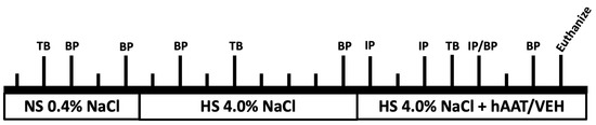
Figure 1. Fasting blood glucose of the pigs in two groups. Here, 48 days after STZ administration, the blood glucose of pigs in the diabetes group rose higher than average and was kept at a high level until 90 days (** p < 0.01; *** p < 0.001).
Figure 1. Fasting blood glucose of the pigs in two groups. Here, 48 days after STZ administration, the blood glucose of pigs in the diabetes group rose higher than average and was kept at a high level until 90 days (** p < 0.01; *** p < 0.001).
Figure 2. (A) BSE image processing and analysis workflow. Step 1. BSE Images were binarized by the internode global thresholding of Image J software. Step 2. Clear images were obtained by filling little holes and removing little noises to identify lacunar osteocytes. Step 3. Porosity identification was fulfilled to separate osteocyte lacunae from other objects. (B) The midpoint line of the histogram of image intensity value was used as the thresholding line for the image threshold.
Figure 2. (A) BSE image processing and analysis workflow. Step 1. BSE Images were binarized by the internode global thresholding of Image J software. Step 2. Clear images were obtained by filling little holes and removing little noises to identify lacunar osteocytes. Step 3. Porosity identification was fulfilled to separate osteocyte lacunae from other objects. (B) The midpoint line of the histogram of image intensity value was used as the thresholding line for the image threshold.
Figure 3. (A) The original image. (B) The binary image. (C) A picture of all objects has been demonstrated for object segmentation. (D) Classification criteria for object segmentation. The area histogram of all objects is shown by the location of all the objects. Objects less than 8 µm2 in size are defined as noises. To obtain the actual maximal area boundary line of the osteocyte lacunae, objects with an area between 100 µm2 and 500 µm2 were segmented into a separate image every 50 µm2 to be compared with the original image to make sure of the exact value to define the osteocyte lacunae area. This process is repeated 24 times because three images are selected from every sample. There are four samples in each group used for observation by BSE. Finally, 280 µm2, the average value of 24 images, is set as the maximal boundary line of the osteocyte lacunae. Objects with an area larger than 280 µm2 were defined as other canals, which include blood vessels, Haver’s channels, and others.
Figure 3. (A) The original image. (B) The binary image. (C) A picture of all objects has been demonstrated for object segmentation. (D) Classification criteria for object segmentation. The area histogram of all objects is shown by the location of all the objects. Objects less than 8 µm2 in size are defined as noises. To obtain the actual maximal area boundary line of the osteocyte lacunae, objects with an area between 100 µm2 and 500 µm2 were segmented into a separate image every 50 µm2 to be compared with the original image to make sure of the exact value to define the osteocyte lacunae area. This process is repeated 24 times because three images are selected from every sample. There are four samples in each group used for observation by BSE. Finally, 280 µm2, the average value of 24 images, is set as the maximal boundary line of the osteocyte lacunae. Objects with an area larger than 280 µm2 were defined as other canals, which include blood vessels, Haver’s channels, and others.
Figure 4. (A) The original image. (B) The image with small cracks that have been wrongly identified as osteocyte lacunae after the segmentation of objects in BSE images. These cracks are marked in the red circle. (C) The small cracks have been correctly removed from the osteocyte lacunae to be other canals. These cracks are marked in the red circle. (D) Classification criteria for the removal of small cracks from the osteocyte lacunae. A histogram of the parameter of Circ. of all objects is demonstrated. To obtain the specific minor Circ. boundary line of the osteocyte lacunae, objects of Circ. from 0 to 0.5 are segmented to a separate the images every 0.1 to compare with the original image to make sure which value is the exact value for defining the osteocyte lacunae. This process is repeated 24 times because 24 images are selected from two groups, as shown in picture D. Finally, 0.34, the average value, is set as the minimal boundary line of osteocyte lacunae. Objects with the parameter of Circ. less than 0.34 are defined as small cracks.
Figure 4. (A) The original image. (B) The image with small cracks that have been wrongly identified as osteocyte lacunae after the segmentation of objects in BSE images. These cracks are marked in the red circle. (C) The small cracks have been correctly removed from the osteocyte lacunae to be other canals. These cracks are marked in the red circle. (D) Classification criteria for the removal of small cracks from the osteocyte lacunae. A histogram of the parameter of Circ. of all objects is demonstrated. To obtain the specific minor Circ. boundary line of the osteocyte lacunae, objects of Circ. from 0 to 0.5 are segmented to a separate the images every 0.1 to compare with the original image to make sure which value is the exact value for defining the osteocyte lacunae. This process is repeated 24 times because 24 images are selected from two groups, as shown in picture D. Finally, 0.34, the average value, is set as the minimal boundary line of osteocyte lacunae. Objects with the parameter of Circ. less than 0.34 are defined as small cracks.
Figure 5. Micro-CT analysis of two groups. A total of six samples of the jaw bone, including three in the control group and three in the diabetes were prepared for the micro-CT scan. Three cubes (0.344 cm × 0.344 cm × 0.344 cm) of bone within the tooth root bifurcation area were selected for analysis in every sample.
Figure 5. Micro-CT analysis of two groups. A total of six samples of the jaw bone, including three in the control group and three in the diabetes were prepared for the micro-CT scan. Three cubes (0.344 cm × 0.344 cm × 0.344 cm) of bone within the tooth root bifurcation area were selected for analysis in every sample.
Figure 6. Osteocyte lacunar morphometric properties of the area and perimeter. (A) Properties of area. The interquartile range (IQR), range, and median lacunae area (µm2). Control group vs. diabetes group: IQR = 20.293–65.741 vs. 18.262–53.499; range = 9.049–279.401 vs. 9.131–278.515; median = 38.006 vs. 31.15 (p < 0.0001, Mann–Whitney test). (p < 0.0001, Kolmogorov–Smirnov test). (B) Distribution line of the area in diabetes and control groups. (C) Lacunae area cumulative frequency distribution. The cumulative frequency distribution of the control is below that of the diabetes group. (D) Properties of the perimeter. The interquartile range (IQR), range, and median lacunae perimeter (µm). Control group vs. Diabetes group: IQR = 16.87–32.63 vs. 15.32–29.61; range = 9.513–97.55 vs. 9.555–96.62; median = 23.62 vs. 21.27 (p < 0.0001, Mann–Whitney test). (p < 0.0001, Kolmogorov–Smirnov test). (E) Distribution line of the perimeter of lacunae in the diabetes group and control group. (F) Perimeter cumulative frequency distribution of lacunae. The cumulative frequency distribution of the control is below that of the diabetes group. (**** p < 0.0001).
Figure 6. Osteocyte lacunar morphometric properties of the area and perimeter. (A) Properties of area. The interquartile range (IQR), range, and median lacunae area (µm2). Control group vs. diabetes group: IQR = 20.293–65.741 vs. 18.262–53.499; range = 9.049–279.401 vs. 9.131–278.515; median = 38.006 vs. 31.15 (p < 0.0001, Mann–Whitney test). (p < 0.0001, Kolmogorov–Smirnov test). (B) Distribution line of the area in diabetes and control groups. (C) Lacunae area cumulative frequency distribution. The cumulative frequency distribution of the control is below that of the diabetes group. (D) Properties of the perimeter. The interquartile range (IQR), range, and median lacunae perimeter (µm). Control group vs. Diabetes group: IQR = 16.87–32.63 vs. 15.32–29.61; range = 9.513–97.55 vs. 9.555–96.62; median = 23.62 vs. 21.27 (p < 0.0001, Mann–Whitney test). (p < 0.0001, Kolmogorov–Smirnov test). (E) Distribution line of the perimeter of lacunae in the diabetes group and control group. (F) Perimeter cumulative frequency distribution of lacunae. The cumulative frequency distribution of the control is below that of the diabetes group. (**** p < 0.0001).
Figure 7. Osteocyte lacunar morphometric properties of the roundness and aspect ratio. (A) Properties of roundness. The interquartile range (IQR), range, and median lacunae area (µm2). Control group vs. diabetes group: IQR = 0.466–0.7113 vs. 0.466–0.706; range = 0.142–1 vs. 0.164–1; median = 0.5905 vs. 0.5899 (p = 0.9439, Mann–Whitney test). (p = 0.2368, Kolmogorov–Smirnov test). (B) Distribution line of lacunae roundness in the diabetes group and control group. (C) Cumulative frequency distribution of lacunae roundness. No noticeable difference can be seen between the two groups. (D) Properties of aspect ratio. The interquartile range (IQR), range, and median lacunae aspect ratio. Control group vs. diabetes group: IQR = 1.406–2.148 vs. 1.416–2.148; range = 1–7.051 vs. 1–6.089; median = 1.867 vs. 1.869 (p = 0.9431, Mann–Whitney test). (p = 0.2368, Kolmogorov–Smirnov test). (E) Distribution line of the aspect ratio in the diabetes group and control group. (F) Cumulative frequency distribution of the lacunae aspect ratio. No obvious difference can be seen between the two groups.
Figure 7. Osteocyte lacunar morphometric properties of the roundness and aspect ratio. (A) Properties of roundness. The interquartile range (IQR), range, and median lacunae area (µm2). Control group vs. diabetes group: IQR = 0.466–0.7113 vs. 0.466–0.706; range = 0.142–1 vs. 0.164–1; median = 0.5905 vs. 0.5899 (p = 0.9439, Mann–Whitney test). (p = 0.2368, Kolmogorov–Smirnov test). (B) Distribution line of lacunae roundness in the diabetes group and control group. (C) Cumulative frequency distribution of lacunae roundness. No noticeable difference can be seen between the two groups. (D) Properties of aspect ratio. The interquartile range (IQR), range, and median lacunae aspect ratio. Control group vs. diabetes group: IQR = 1.406–2.148 vs. 1.416–2.148; range = 1–7.051 vs. 1–6.089; median = 1.867 vs. 1.869 (p = 0.9431, Mann–Whitney test). (p = 0.2368, Kolmogorov–Smirnov test). (E) Distribution line of the aspect ratio in the diabetes group and control group. (F) Cumulative frequency distribution of the lacunae aspect ratio. No obvious difference can be seen between the two groups.
Figure 8. Osteocyte lacunar morphometric properties of the density. (A) The formula for density calculation is given. There is no significant difference between the two groups. (B) The segmentation of lacunae and other canals is shown.
Figure 8. Osteocyte lacunar morphometric properties of the density. (A) The formula for density calculation is given. There is no significant difference between the two groups. (B) The segmentation of lacunae and other canals is shown.
Figure 9. Properties of the area, perimeter, roundness, and aspect ratio from analysis 1 and analysis 2. (A) The area of osteocyte/lacunae in both analysis 1 and analysis 2 shows a significant difference between the control group and the diabetes group (p < 0.0001, Mann–Whitney test). (B) The perimeter of osteocyte/lacunae in both analysis 1 and analysis 2 shows a significant difference between the control group and the diabetes group (p < 0.0001, Mann–Whitney test). (C) The roundness of the osteocyte/lacunae in both analysis 1 and analysis 2 shows no significant difference between the control group and diabetes group (analysis 1, p = 0.944, Mann–Whitney test; analysis 2, p = 0.610, Mann–Whitney test). (D) The perimeter of aspect ratio in both analysis 1 and analysis 2 shows no significant difference between the control group and the diabetes group (analysis 1, p = 0.943, Mann–Whitney test; analysis 2, p = 0.608, Mann–Whitney test) (**** p < 0.0001).
Figure 9. Properties of the area, perimeter, roundness, and aspect ratio from analysis 1 and analysis 2. (A) The area of osteocyte/lacunae in both analysis 1 and analysis 2 shows a significant difference between the control group and the diabetes group (p < 0.0001, Mann–Whitney test). (B) The perimeter of osteocyte/lacunae in both analysis 1 and analysis 2 shows a significant difference between the control group and the diabetes group (p < 0.0001, Mann–Whitney test). (C) The roundness of the osteocyte/lacunae in both analysis 1 and analysis 2 shows no significant difference between the control group and diabetes group (analysis 1, p = 0.944, Mann–Whitney test; analysis 2, p = 0.610, Mann–Whitney test). (D) The perimeter of aspect ratio in both analysis 1 and analysis 2 shows no significant difference between the control group and the diabetes group (analysis 1, p = 0.943, Mann–Whitney test; analysis 2, p = 0.608, Mann–Whitney test) (**** p < 0.0001).
Figure 10. (A,D) The osteocyte lacunae morphology in acid-etched samples using BSE in two groups. The pericellular area was demonstrated in the high magnification of the BSE image. (B,E) The binary picture after thresholding; the edge of the peri-lacunae area can be observed obviously. (C,F) The location of osteocytes and lacunae for analysis. (G) The size of osteocytes is significantly decreased in the diabetes group (p = 0.0003 < 0.001, Mann–Whitney test). (H) The lacunae area is considerably reduced in the diabetes group (p = 0.0002 < 0.001, Mann–Whitney test). (I) The pericellular area is reduced to a small extent in the diabetes group. This difference also has a statistical significance (p = 0.0164 < 0.005, Mann–Whitney test; * p < 0.05; *** p < 0.001).
Figure 10. (A,D) The osteocyte lacunae morphology in acid-etched samples using BSE in two groups. The pericellular area was demonstrated in the high magnification of the BSE image. (B,E) The binary picture after thresholding; the edge of the peri-lacunae area can be observed obviously. (C,F) The location of osteocytes and lacunae for analysis. (G) The size of osteocytes is significantly decreased in the diabetes group (p = 0.0003 < 0.001, Mann–Whitney test). (H) The lacunae area is considerably reduced in the diabetes group (p = 0.0002 < 0.001, Mann–Whitney test). (I) The pericellular area is reduced to a small extent in the diabetes group. This difference also has a statistical significance (p = 0.0164 < 0.005, Mann–Whitney test; * p < 0.05; *** p < 0.001).
Figure 11. The micro−CT results show no significant difference between the diabetic group and the control group. (A) The trabecular thickness shows no significant difference (nested t-test, p = 0.3200). (B) The space between the trabecular bone has no significant difference (nested t-test, p = 0.0751). (C) The trabecular number shows no significant difference (nested t-test, p = 0.7655). (D) The structure model index shows no significant difference (nested t-test, p = 0.2155). (E) The bone volume under the same total volume shows no significant change (nested t-test, p = 0.1485). (F) The trabecular surface area under the same volume shows no significant change (nested t-test, p = 0.2465).
Figure 11. The micro−CT results show no significant difference between the diabetic group and the control group. (A) The trabecular thickness shows no significant difference (nested t-test, p = 0.3200). (B) The space between the trabecular bone has no significant difference (nested t-test, p = 0.0751). (C) The trabecular number shows no significant difference (nested t-test, p = 0.7655). (D) The structure model index shows no significant difference (nested t-test, p = 0.2155). (E) The bone volume under the same total volume shows no significant change (nested t-test, p = 0.1485). (F) The trabecular surface area under the same volume shows no significant change (nested t-test, p = 0.2465).
留言 (0)