Here, we describe an approach to estimate genetic penetrance for autosomal dominant traits using population-scale data.

Our method builds upon and extends an existing disease model [16] which makes the following assumptions: in a nuclear family, a rare dominant pathogenic variant is necessary but not sufficient for disease to occur, therefore penetrance, denoted \(f\), is not complete and family members who do not harbour the variant are not affected; all variants are inherited from exactly one parent, thus there are no people homozygous for the variant or de novo variants. Our extended model relaxes the assumption that the variant is necessary for disease to occur: it assumes that people not harbouring the variant have a residual risk for developing disease after accounting for the proportion of disease occurrences attributed to the variant, denoted \(g\).

Accordingly, if the probability of an individual being affected by a disease, \(P(A)\), is \(f\) when harbouring variant \(M\) or \(g\) if \(M\) is absent, denoted \(^}\), \(P(A)\) can be determined by considering the probability of harbouring \(M\), \(P(M)\):

$$P\left(A\right)=f\times P\left(M\right)+g\times P\left(^}\right),$$

(1)

letting \(P\left(M\mathrm}\right)=1-P\left(M\right)\).

In a family where a single parent harbours, and each child has a 0.5 chance of inheriting, \(M\), the following probabilities of being affected can be determined per family member:

for the variant harbouring parent, where \(P(M)=1\);

for each offspring, each of whom has \(P(M)=0.5\), and thus risk influenced by both \(f\) and \(g\); and

for the parent without \(M\), where \(P(M)=0\), and therefore for whom disease risk is only determined by that which is associated with \(^}\).

Considering these individual disease probabilities, three probabilities can be determined for a nuclear family where one parent harbours a given variant: that no family members are affected, \(P(unaffected)\); that exactly one member is affected, \(P(sporadic)\); and that more than one member is affected, \(P(familial)\). These probabilities are determined by penetrance, \(f\), residual disease risk \(g\) if not harbouring the variant, and sibship size, \(N\). In a family with \(N\) siblings:

$$P\left(unaffected\right)=\left(1-f\right)-\frac\right)}^\left(1-g\right) ,$$

(5)

where no family member, with or without the variant, develops the disease, and where each of the sibs has \(^\!\left/ \!_\right.\) probability of being transmitted the variant.

$$P\left(sporadic\right)=-\frac\right)}^\left(1-g\right)+\left(1-f\right)N\left(\frac+\frac\right)-\frac\right)}^\left(1-g\right)+(1--\frac\right)}^g ,$$

(6)

if one family member develops the disease. This may be either may be the variant-harbouring parent, exactly one of the sibs, or the parent not harbouring the variant (on account of residual risk \(g\)). Then,

$$P\left(familial\right)=1-P\left(unaffected\right)-P\left(sporadic\right)=1-\left(\begin\left(1-f\right)-\frac\right)}^\left(1-g\right)+\\ -\frac\right)}^\left(1-g\right)+\\ \left(1-f\right)N\left(\frac+\frac\right)-\frac\right)}^\left(1-g\right)+\\ (1--\frac\right)}^g\end\right) ,$$

(7)

where two or more family members develop the disease, which can be determined from \(P(unaffected)\) and \(P(sporadic)\) since the total probability of a family being unaffected, sporadic, or familial must sum to 1.

If \(g=0\), the original [16] and extended models are equivalent.

Conversely, penetrance can be estimated given the observed rates of the unaffected, sporadic, and familial disease states in families where the pathogenic variant occurs, the average sibship size for these families, and an estimate of residual disease risk \(g\). We can also estimate penetrance based on the observed rates of families presenting as unaffected versus affected, a fourth disease state whereby

$$P\left(affected\right)=P\left(familial\right)+P\left(sporadic\right) .$$

(8)

The observed rate of the arbitrarily-labelled disease state ‘X’, \(R^\), is used to indicate the frequency of one of the sampled disease states across all states sampled. \(R^\) can be specified for any valid combination of the four disease states, drawing from any two or three of the familial, sporadic, and unaffected disease states, or from the affected and unaffected states. Data from the affected state cannot be specified alongside that of the familial or sporadic disease states since the former is determined through their combination. \(R^\) may be specified directly if the distribution of disease states across people with the variant is known for the state-combination used or derived as a weighted proportion of estimates of heterozygous variant frequency across people with and without the variant (see Table 1).

Sibship size can be estimated for the sample either directly, based on the average sibship size among sampled families, or indirectly, by designating an estimate representative of the sample (e.g. from global databases).

Under Bayes theorem [18], \(g\) can be determined from \(P(A)\) and \(P(M)\) within the general population, respectively \(P^\) and \(P^\), and the frequency of variant \(M\) among people affected by disease, \(_\):

$$g=\frac^\times \left(1-_\right)}^\right)}.$$

(9)

\(_\) and \(P^\) may each be determined by weighted sums:

$$_=_\times P\left(F|A\right)+_\times P\left(S|A\right) ,$$

(10)

and

$$P^=_\times P^+_\times \left(1-P^\right) ,$$

(11)

where \(_\) denote the variant frequencies in the familial, sporadic, and unaffected states, \(P(F|A)\) is the rate at which people in the affected population, \(A\), are familial, and \(P(S|A)\) is the disease sporadic rate (\(P(S|A)=1-P(F|A)\)). If the disease is rare in the population, \(g\approx 0\) and has a negligible influence upon penetrance estimates (see the simulation studies in Additional File 1: Sect. 1.2.3).

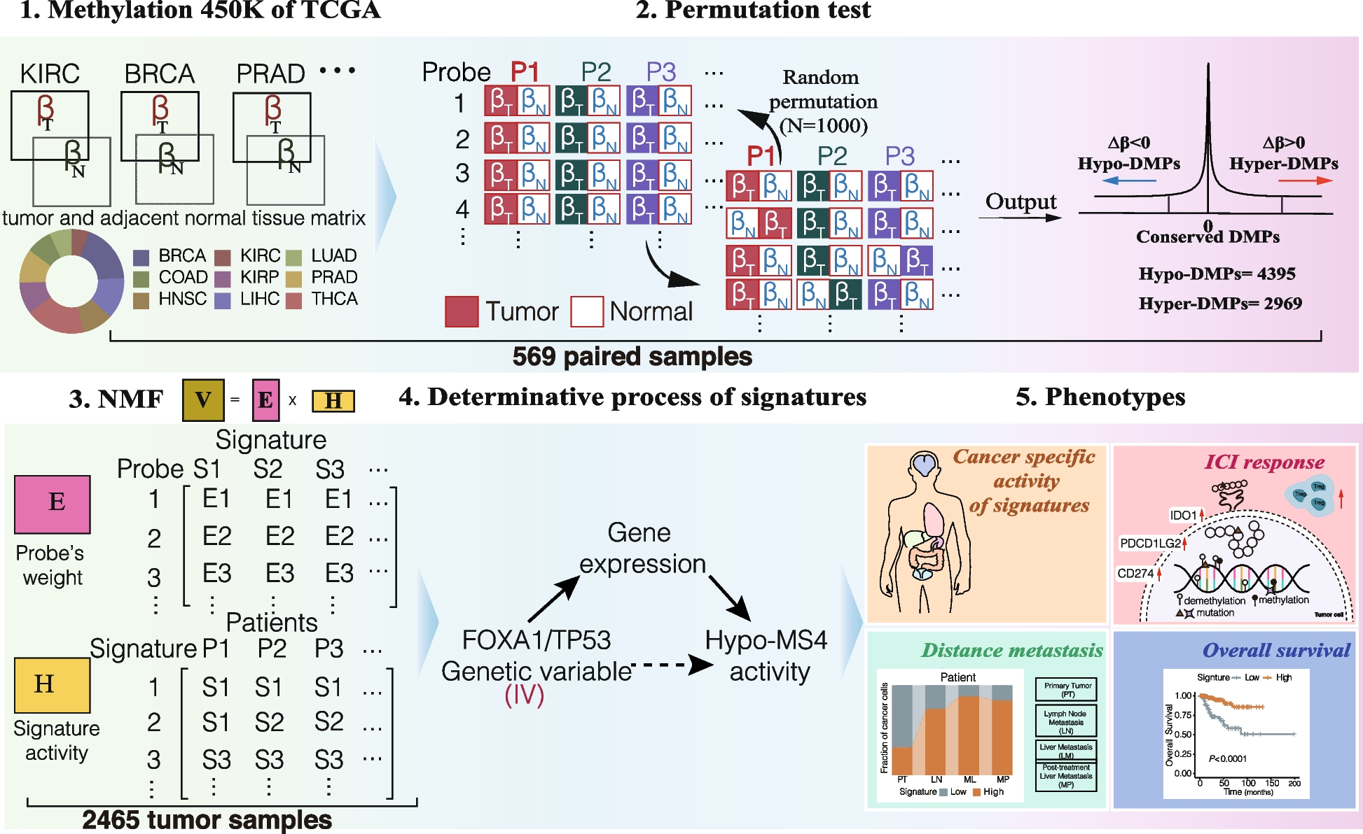
Our penetrance calculation method involves four steps and includes the option to derive error in the estimate. These processes are summarised in Fig. 1 and comprehensively outlined in Additional File 1: Sect. 1.1.

Summary of the key steps within this penetrance estimation approach. Legend: Step 1: Variant frequencies (M) and weighting factors (W) are defined for a valid subset of the familial (F), sporadic (S), unaffected (U), and affected (A) states (see Table 1) to calculate rate of one of these states, arbitrarily labelled state X, among families harbouring the pathogenic variant across those states with data provided, \(R^\). Step 2: Eqs. (5–8) are applied to calculate \(P(familial)\), \(P(sporadic)\), \(P(unaffected)\), and \(P(affected)\), for a series of penetrance values, \(f_=0,\dots ,1\), at a defined sibship size, \(N\), and with disease risk \(g\) for people not harbouring the variant. The rate of state X expected at each \(f_\) among variant harbouring families from those states represented in Step 1, \(R_^\), is calculated and stored alongside the corresponding \(f_\) in a lookup table. Step 3: The lookup table is queried using \(R^\) to identify the closest \(R_^\) value and corresponding \(f_\). Step 4: Bias in the obtained \(f_\) estimate is corrected by simulating a population of families representative of the sample data, estimating the difference between true and estimated penetrance values in this population between \(f=0,\dots ,1\) and adjusting the estimated \(f_\) by error predicted within a polynomial regression model fitted upon the simulated estimate errors. Optional step: Confidence intervals for \(R^\) can be calculated from error in the estimates of \(M\) provided [48]; Penetrance is estimated as in Steps 3 and 4 for the interval bounds. All steps within this approach are comprehensively detailed in Additional File: Sect. 1.1

The method assumes that: one person is sampled per family and disease states are assigned based on the status of the person sampled and first-degree family members only; all variants are inherited from exactly one parent and there are no de novo variants; the value specified for sibship size is representative of sibship size across disease state groups. We recommend providing an estimate of \(g\), however, \(g=0\) by default, which makes the additional assumption that the trait only occurs in members of sampled families owing to the presence of the variant.

A further assumption is made in each of the two scenarios for determining \(R^\). When sampling across only families where the variant occurs, it is assumed that disease state classifications for sampled families will not change at a future time. When estimating variant frequencies within disease states across cohorts of people with and without the variant, it is assumed that family disease states change comparably over time for people with and without the variant. The latter assumption can be partially tested by examining whether age of disease onset is equally variable for people with and without the tested variant; the assumption is further discussed in Additional File 1: Sect. 1.2.2.

Additional File: Sect. 1.2 outlines the steps taken for approach validation, including details of several simulation studies and comparison between using a lookup table or maximum-likelihood approach for Step 3. The included simulation studies test accuracy in penetrance estimation when input parameters are correctly or incorrectly specified, when \(g\) is accurately measured or assumed to be 0, and according to age of sampling across several scenarios.

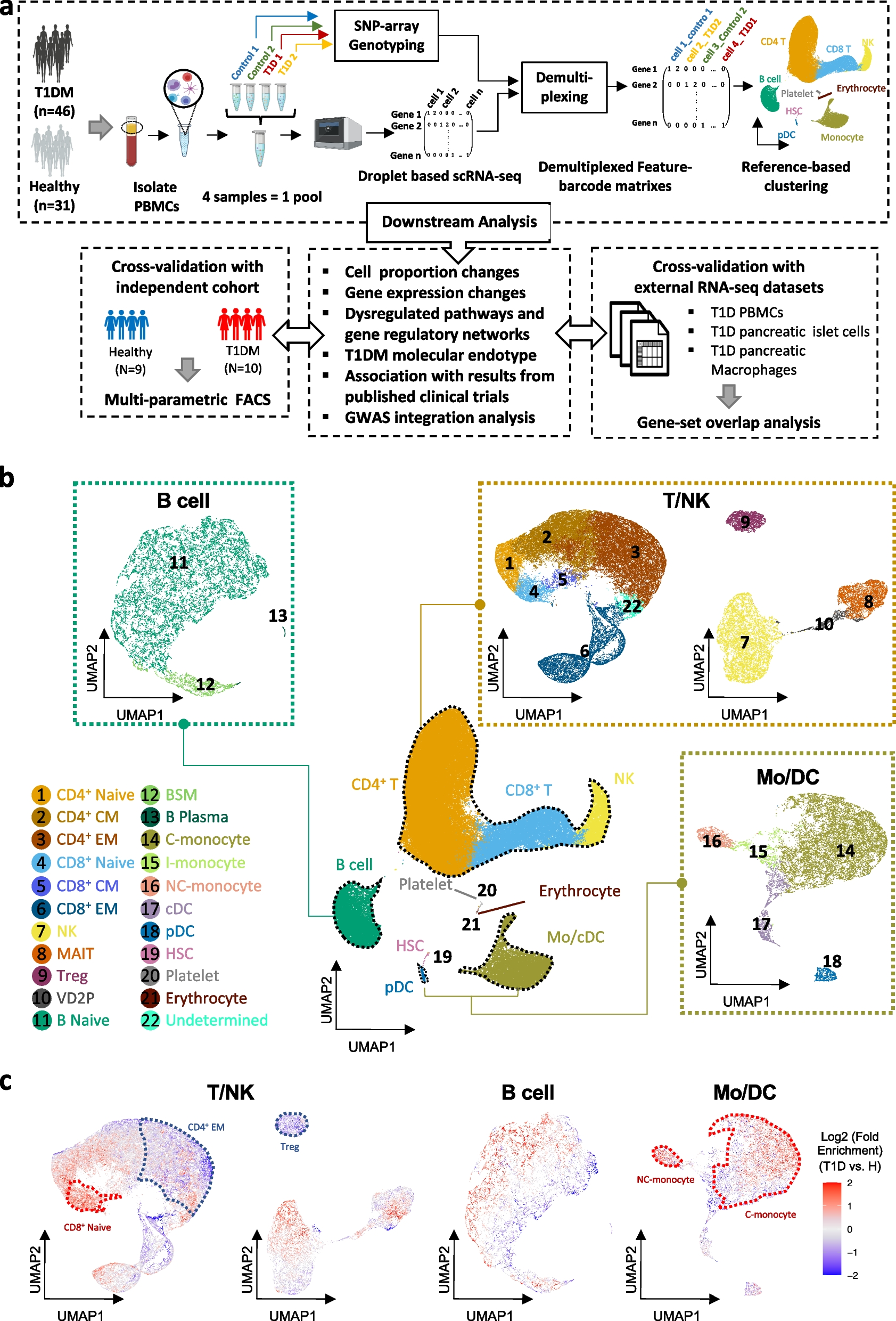
We have made this approach available as the R function adpenetrance hosted on GitHub [19]. In the GitHub repository, we additionally provide functions to calculate \(g\); test for equal onset variability across two groups; and simulate how a certain degree of unequal onset variability, as indicated by the previous function, may affect penetrance estimates. To facilitate easy use, the approach is also hosted on a publicly available web-server, developed using the R Shiny package (version 1.7.3) [20, 21]. The web tool is further described in the Additional File: Sect. 1.3, and Fig. 2 presents an example of its usage.

Example interface and output of the ADPenetrance web tool [20]. Legend: Here we show the example of penetrance of SOD1 variants for amyotrophic lateral sclerosis in a European population, applying variant frequency estimates for familial and sporadic ALS patients of European ancestry, an estimate of ALS disease risk among people not harbouring SOD1 variants, and the average Total Fertility Rate for the European Union in 2018 [22, 35]

Input parameters for included case studies were estimated using publicly available data. Variant frequencies were estimated across people with and without the variant in the familial, \(_\), and sporadic, \(_,\) states in all cases and, in case 1, the unaffected state, \(_\). \(_\) was integrated into penetrance estimation for case study 1 only to demonstrate the application of the method when sampling from various disease state combinations. This was not applied to other case studies as estimation focusses upon rare variants liable to ascertainment bias in control populations. In all cases, we derived the standard error of these values, \(__}}\), to allow for assessment of error in the penetrance estimate. Variant frequency estimates were weighted to calculate \(R^\) among variant-harbouring families from those states modelled using the factors presented in Table 1. Accordingly, \(P(F|A)\) and \(P(S|A)\) were defined as weighting factors in all cases. \(P^\) is used in all case studies to derive \(g\), according to Eqs. (9–11), and is used as a weighting factor in case 1 only.

Sibship size, \(N\), was estimated in each case based on the Total Fertility Rates reported in the World Bank database [22] for the world region(s) best representing the sample.

An R script permitting replication of each case study is provided within our GitHub repository (see the ‘Availability of data and materials’ [19]).

We estimated the penetrance of the LRRK2 p.Gly2019Ser variant for PD. This case illustrates the flexibility of this method for application using data drawn from several combinations of the defined disease states.

The first-degree familiality rate of PD, about \(0.105\), was used to estimate \(P(F|A)\) and \(P(S|A)\) [23, 24]. \(P^\) was estimated as \(1\) in \(37\) (\(0.027\)), the lifetime risk of developing PD [25].

We estimated \(_\) using data aggregated from 18 European ancestry groups within a sample of \(24\) world populations [26]. Of \(\mathrm\) unrelated people with familial PD manifestations, \(126\) (\(_=0.033, __}}=2.92\times ^\)) harboured the LRRK2 p.Gly2019Ser variant, compared to \(130\) of \(\mathrm\) with sporadic PD (\(_=0.012, __}}=1.04\times ^\)).

As LRRK2 p.Gly2019Ser occurred in only \(2\) members of the unaffected control sample, we estimated \(_\) using the larger European (non-Finnish) sample of the gnomAD v2.1.1 (controls) database [27], in which \(10\) of \(\mathrm\) people harboured the variant (\(_=4.67\times ^, __}}=1.47\times ^\)).

We estimated that \(g=0.0267\), in accordance with Eqs. (9–11), based on the estimated \(_\), \(P(A)\), and \(P\left(F|A\right).\)

As no single region is representative of the total sample, we estimated that \(N=1.572\) by aggregating Total Fertility Rate estimates available in the World Bank database [22] across each of the 18 European populations sampled, weighted by the proportional contribution of each population to the sample (see Additional File 1: Table S1) [26].

Additional region-specific and joint population penetrance estimates for this variant are presented in Additional File 1: Table S2.

We estimated the penetrance of variants in the BMPR2 gene for heritable PAH, a gene for which the low penetrance of pathogenic variants is well established [28].

Input parameters were defined based on only people with idiopathic (sporadic) or heritable PAH diagnoses [17]. This captures people with and without family disease history and excludes PAH manifestations associated with comorbidities or drug exposure.

We estimated \(P(F|A)\) and \(P\left(S|A\right)\) using the first-degree familiality rate of heritable PAH, about \(0.055\) of people affected by either idiopathic or familial PAH [28]. \(P^\) was estimated as \(1\) in \(20\) (\(0.05\)), according to an estimated \(1\) in \(10\) lifetime risk of developing any PAH, and that idiopathic and heritable PAH forms account for approximately \(50\%\) of PAH occurrences [28,29].

To minimise any study-specific bias, we applied data from two reports to build independent estimates for each of \(_\). The first dataset [17], includes \(247\) people with familial PAH, of which \(202\) harboured BMPR2 variants (\(_=0.818, __} }=0.025\)), compared to \(200\) of \(1174\) in the sporadic state (\(_=0.170, __}}=0.011\)). The second dataset [30] identified that \(40\) of \(58\) people with familial PAH (\(_=0.690, __} }=0.061\)) harboured BMPR2 variants, compared to \(26\) of \(126\) in the sporadic state (\(_=0.206, __}}=0.036\)). Variant counts were additionally reported separately for small genetic variations (single nucleotide variants and indels) and structural variants in BMPR2, allowing penetrance estimation stratified by variant type. Letting \(_=0\), we estimated that \(g=0.0401\) for dataset 1, and \(g=0.0388\) for dataset 2, in accordance with Eqs. (9–11).

The first dataset may violate two assumptions of our approach: first, information on familial clustering was reportedly unavailable and so some families may be represented more than once in the familial state; second, it is not specified whether disease familiality is defined only by the disease status of first-degree relatives. The second sample overcomes a limitation of the first as each family is represented only once in variant counts. However, it is not reported whether disease states are defined according to the status of first-degree relatives only. As \(R^\) is calculated after weighting \(_\) by the first-degree familial disease rate, the impact of some bias in variant frequency estimates upon penetrance estimates will be minimised.

The first cohort samples people from Asian, European, and North American populations; French, German and Italian cohorts comprise about 60% of the sample [17]. The second cohort samples people exclusively from Western Europe [30]. We therefore estimated that \(N=1.543\) in both instances, the Total Fertility Rate of the European Union in 2018 [22].

We estimated the penetrance of variants in the SOD1 and C9orf72 genes for ALS. For SOD1, we examined the aggregated penetrance of SOD1 variants harboured by people with ALS. For C9orf72, we examined the penetrance of a single pathogenic variant, a hexanucleotide GGGGCC repeat expansion (C9orf72RE; g.27573529_27573534GGCCCC[30 <]). These penetrances have been historically difficult to establish without incurring kinship-specific biases. They represent ideal candidates for application of our method.

The first-degree familiality rate of ALS, about \(0.050\), was applied to define \(P(F|A)\) and \(P(S|A)\) in these cases [31, 32]. \(P^\) was estimated as \(1\) in \(400\) (0 \(.0025\)), the lifetime risk of developing ALS [33].

We drew upon the results of two meta-analyses [34, 35] to estimate \(_\) for SOD1 and C9orf72RE. As variant frequencies differed between Asian and European ancestries, we modelled penetrance separately for each group. We derived \(__}}\) using z-score conversion from the 95% confidence intervals (95% CIs) reported: for the arbitrary state X,

$$__} }=\frac_-_^}$$

(12)

where \(z=1.96\) and \(_^\) is the lower 95% CI bound of the estimate \(_\).

In Asian ALS populations: SOD1 variants were harboured by \(0.300\) (\(__} }=0.025\)) of people with familial and \(0.015\) (\(__} }=2.55\times ^\)) with sporadic disease; C9orf72RE was harboured by \(0.04\) (\(__} }=0.010\)) of people with familial and \(0.01\) (\(__} }=5.10\times ^)\) with sporadic disease. In accordance with Eqs. (9–11), and letting \(_=0\), we estimated that \(g=0.00243\) for SOD1, and \(g=0.00247\) for C9orf72.

In Europeans, SOD1 variants were harboured by \(0.148\) (\(__} }=0.017\)) of people with familial and \(0.012\) (\(__} }=2.55\times ^)\) with sporadic disease; C9orf72RE was harboured by \(0.32\) (\(__} }=0.020\)) of people with familial and 0.05 (\(__} }=5.10\times ^)\) with sporadic disease. In accordance with Eqs. (9–11), and letting \(_=0\), we estimated that \(g=0.00245\) for SOD1, and \(g=0.00234\) for C9orf72.

The SOD1 meta-analysis allowed consideration of the extended kinship when defining familial ALS. The familiality definition used in the C9orf72 analysis is not stated. As before, the weighting of \(_\) by the first-degree familial disease rate when calculating \(R^\) will minimise any impact of some bias in variant frequencies upon penetrance estimates.

We tested for equal onset variability (see Additional File 1: Sect. 1.2.2) with the checkOnsetVariability R function provided in the associated GitHub repository [19], comparing variability in age of ALS onset for people with SOD1 or C9orf72 variants to that of people without variants in these genes. The results (see Additional File 1: Fig. S4) suggested approximately equal onset variability between the SOD1 and no (SOD1 or C9orf72) variant groups, indicated by visual inspection of the cumulative density plot provided and by an approximately equal time spanned between the first and third quartiles of age of onset across the groups. Onset variability appears more unequal in the C9orf72 case study, with a ~ 1.36 times shorter interquartile interval for people harbouring C9orf72RE than the no variant cohort. One of the simulation studies presented in Additional File 1: Sect. 1.2.3; Fig. S11 models a comparable departure from the equal onset variability and demonstrates that a small but tolerable inflation of penetrance estimates may occur if sampling a younger cohort. Since the present penetrance estimates are based on pooled variant frequency estimates from large meta-analyses of variant frequencies in these genes, the present degree of unequal onset variability is unlikely to have impacted penetrance estimation.

In these datasets, the Asian ancestry cohorts were predominantly individuals from East Asia, with small proportion from South Asia. The European ancestry cohorts primarily comprise people from European countries, with some from North America and Australasia. Accordingly, \(N\) was estimated for the Asian population samples as \(1.823\), the Total Fertility Rate for East Asia and Pacific in 2018, and for the European population as \(1.543\), the Total Fertility Rate for the European Union in 2018 [22].