Introduction

Elucidating gene regulatory networks (GRNs) is a fundamental challenge in molecular biology (Hughes et al., 2000). High-throughput technologies provided a wealth of gene expression data which are helpful to interrogate the complex regulatory dynamics inherent to organisms (Algabri et al., 2022; Wang and Liu, 2022). The network structure with genes (genes) and regulatory interactions (edges) can be inferred from the observed data through minimizing the effects of noise and hidden genes (Baruch and Albert-László, 2013; Yang et al., 2022). To improve the accuracy of network reconstruction, various methods have been developed for the reconstruction of GRNs from gene expression profiles (Riet and Kathleen, 2010; Zhang et al., 2022). However, each method has its own strengths and weaknesses (Daniel et al., 2010). Among the methods for GRN inference, most of them are insufficient in determining the causalities or regulatory directions (Krouk et al., 2013; Ahmed et al., 2018). Understanding the causality in the gene expression data is critical to elucidating the underlying regulatory mechanism of cellular machines (Jiang et al., 2000; Nagoshi et al., 2004; Rubin et al., 2019).

Existing methods to infer the GRNs from gene expression data with the motivation of improving the accuracy and scalability of network inference include model-based approaches and machine learning-based approaches (Madar et al., 2009; Zhang et al., 2013). For the model-based approaches, chemical reaction of transcription and translation, as well as other cellular processes, are described as linear or nonlinear differential equations, in which the parameters represent the regulation strengths of the regulators (Gardner et al., 2003; Honkela et al., 2010). Dynamical system models of differential equations can forecast future system behaviors and characterize formal properties such as stability (Zak et al., 2003; Wang et al., 2022). Furthermore, prior information, such as experimentally verified regulations, can be easily included in these models to improve the accuracy of network inference (Studham et al., 2014; Zhang et al., 2017). Moreover, the model-based methods are found useful to remove possible redundant indirect regulations by forcing sparseness on the model (Hurley et al., 2011; Jiang and Zhang, 2022). However, these models are computationally intractable for large GRNs owing to extensive and explicit parameterization requirements (Karlebach and Shamir, 2008; Tibshirani, 2011). For the machine learning-based approaches, the network is inferred through measuring the dependences or causalities between transcriptional factors and target genes (Khatamian et al., 2018; Deng et al., 2021). Popular methods in this category include mutual information (MI) (Modi et al., 2011), conditional mutual information (CMI) (Zhang et al., 2011), part mutual information (Zhao et al., 2016), Granger causality (Finkle et al., 2018), and maximal information coefficient (Reshef et al., 2011; Kinney and Atwal, 2014). With no explicit mechanistic assumptions, the machine learning-based methods are usually more efficient than the model-based methods in the computational complex (Zhang et al., 2015).

As the most popular methods, MI and CMI evaluate the association between the genes by measuring the entropy of their mutual activities, where a lower entropy for a gene indicates that its activities are less randomly distributed; that is, it is statistically dependent on the activities of other genes (Butte and Kohane, 2000). Specially, MI can characterize nonlinear dependency and deal with thousands of variables (genes) in the presence of a limited number of samples. However, the MI between two variables is a symmetric quantity, and so the MI-based methods generally infer undirected interactions (Aghdam et al., 2015). The ordinary differential equation (ODE)-based methods can be used for inference of causal GRNs, but these methods require rigorous datasets like time-series data (Lu et al., 2021; Yang et al., 2021; Chen and Liu, 2022).

In this study, we develop a method for inferring causal GRNs from genetic knockout data. The activities of the downstream target genes respond to the knockout changes of regulatory genes and are identified accurately by comparing the relative change values of the downstream targets and assigning a weight to the relative change values of each gene. It is helpful to remove the spurious edges in the causal inference of GRNs. We dissect the downstream target genes using CMI, MI, and Taylor formula-based regression to determine the causalities among the downstream targets. We model the hierarchy structure of the downstream targets and determine the causalities in different layers with CMI which is efficient to remove these redundant indirect regulations. Consequently, we determine the correlation in the same layer. At last, we use Taylor formula-based regression to determine the causalities in the same layer. With the process repeating for each regulator, the reconstruction of GRNs is achieved. Our method not only has the advantages of the machine learning-based methods but also can determine the regulatory directions. The results on the DREAM3 and DREAM4 datasets show that our method significantly outperforms the existing method in terms of false-positive rates and accuracy.

MethodsDownstream target identification

As the activity of the regulator can be approximated by the expression level of the gene encoding the regulator, we suppose the gene expression level as regulator activity. Let gi represent the ith gene. Considering a network consisted of n genes, gene expression matrix A denotes the gene expression level under different conditions (samples) which can be measured directly from gene knockout experiments. The knockout experiment is implemented for every gene and the downstream gene response to the knockout of gene through the fluctuations of expression levels. The steady-state levels of genes in the wild-type provide a standard of the gene expression changes. Thus, the gene expression levels of wild-type and knockout experiments of each gene provide the information to identify downstream targets. Matrix A consists of n rows with n steady-state values of knockout experiments, and each row is obtained after deleting one of n genes. The vector Aj=a1j,a2j,⋯anjT stands for the jth column of matrix A, in which aij represents the steady-state level of gene gj after knockout of gene gi. The wild-type file contained n steady-state levels of the unperturbed network. The vector A0=a01,a02,⋯,a0n stands for the wild-type data of each gene, in which a0j denotes the steady-state level of the wild-type of gene gj.

The genes whose steady-state values change as a result of a single-gene knockout are likely to be downstream of the perturbed gene. Most causal relationships owing to the gene knockout could be immediately recognized by 0comparing the steady-state data after gene knockout with wild-type data. We calculate the changes of gene gj response to the knockout of every gene by using the following expression:

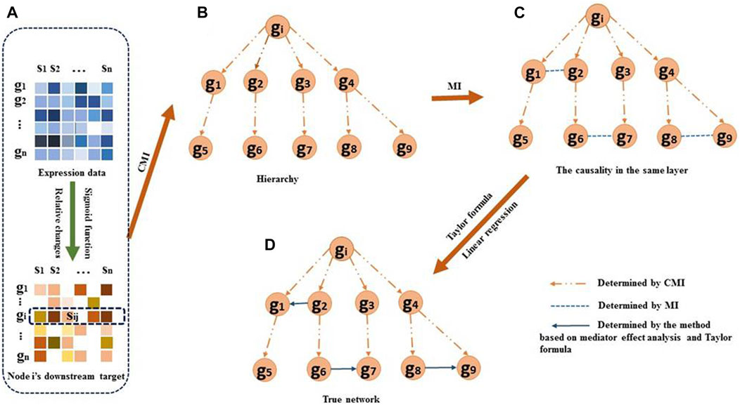
ΔAj=ΔaijT=a1j−a0j,a2j−a0j,⋯,anj−a0jT,(1)

where Δaij=aij−a0j denotes the changes of gene gj by comparing the response to the knockout of gene gi with the wild type. The changes describe the response of all genes as a consequence of the perturbation of the source gene. We use the mean change value to quantify the mean response strengths of the same target to different regulators. The mean change value in gene gj can be expressed as ΔAj¯=1n∑i=1nΔaij. Δaij for different genes varies widely because the wild-type data of different genes vary widely. So we use the relative change value to quantify the response strengths of the same target to different regulators. We obtain the relative change value vector which is ∆S·j=∆s1j,∆s2j⋯∆snjT, where ∆sij=∆aij/∆Aj¯ denotes a relative change value of gene gj. Gene gi is called as the regulator, and the genes that respond to the change of gi are called downstream target genes or targets. aij−a0j of each gene varies widely because the wild-type data of each gene vary widely and because the activities of the downstream target genes responding to the same knock-out change of regulatory gene vary widely. To calculate the activities of the downstream target genes and compare the relative changes of gj with other genes, we assign a weight to ∆S· j by sigmoid function wj=1/1+erbj−u, where parameters r and u describe the coefficients of sigmoid function, and bj=maxi∆aij/a0j describes the maximum response strength of gj to the changes of other genes. Parameters r and u are given but not estimated to balance the computation of w. Parameter r is set as a negative integer number and parameter u is set as a positive number and is smaller than 1. In general, the values chosen will not affect the final results. By calculating S· j=wj∆S· j, we obtain a matrix S=Si,jn×n, where S·j denotes the jth column of matrix S, and the row vector Si · denotes the ith row of matrix S. Given a threshold parameter θ0 for deciding the downstream target genes of regulator gi, the elements in Si · above θ0 are regarded as downstream target genes gi (Figure 1A). Most casual relationships could be accurately recognized from Si ·. Due to the sparseness of GRNs, the downstream targets consist of a small number of genes, which is helpful to remove the indirect dependencies and reduce the computational complexity.

FIGURE 1. Overview of the DDTG method. (A) For each regulator gi, the downstream target genes sij of the regulator are identified by the Sigmoid function and by comparing the relative change values. (B) Hierarchy structure of downstream target genes will be decided by using CMI. Assuming genes g1–g9 are the downstream target genes of regulator gi. As an example, genes g1 and g5 belong to the 2 combination of the downstream target genes. If Igi,g5|g1 is small, it indicates that gi regulates g1 directly and g1 regulates g5 directly. The dashed arrows denote the regulatory direction. (C) The correlations between two genes in the same layer. The dashed lines without arrows denote the genes being strongly dependent on each other. Edges g1–g2, g6–g7, and g8–g9 are directly correlated with each other in the same layer. (D) The regulatory direction between two genes in the same layer is determined using the Taylor formula and linear regression. The solid arrows denote the causality in the same layer. The reconstruction of GRNs is achieved by aggregating the edges from each step.

Causality among hierarchy genes

Some of the downstream targets may be indirectly regulated by gene gi. The remaining task is thus to distinguish direct dependence from indirect dependence. To accomplish this, we use conditional mutual information (CMI) to discriminate the genes directly regulated by gi from the genes indirectly regulated by gi. Accordingly, we obtain a hierarchy structure of the downstream targets of gi. So the topological structure of the downstream target genes of gi is a two-layer network. The genes in the first layer are directly regulated by regulator gi, and the genes in the second layer are indirectly regulated by gi.

The CMI allows measuring the dependency of two genes in the context of a third gene. We assume that gj and gk are gi’s downstream target genes. The interaction between gene gi and gj can be measured in the context of gene gk by the CMI, which is defined as follows:

Igi,gj|gk=∑x∈gi, y∈gj, z∈gkpx,y,zlogpx,y|zpx|zpy|z

The CMI can be easily calculated using the following equation:

Igi,gj|gk=12logCgi,gk⋅Cgj,gkCgk⋅Cgi,gj,gk,(2)

where C is the covariance matrix of variables, and C is the determinant of matrix C. If gj and gk carry the same information about gi, Igi,gj|gk=0. It indicates that gi directly regulates gk and gi indirectly regulates gj mediated by gk; that is, gene gk directly regulates gene gj. The genes regulated directly by gi form a layer, namely, the first layer, and the genes regulated indirectly by gi form a layer, namely, the second layer (Figure 1B).

Correlations among the genes in the same layer

For the genes in the same layer, the correlations among them are measured by mutual information (MI). MI between two genes gh and gl can be defined as follows (Altay and Emmert-Streib, 2010):

Igh,gl=−∑x∈gk,y∈glpx,ylogpx,ypxpy

The MI can be easily calculated using the following equivalent formula:

Igh,gl=12logCgh⋅CglCgh,gl,(3)

where C is the covariance matrix of variables, and C is the determinant of matrix C. If Igh,gl is large, it indicates that a strong dependency exists between genes gh and gl (Figure 1C).

Regulatory directions between genes in the same layer

To determine if the regulatory direction in the scenario of gh and gl is in the same layer and a strong dependency exists between them, we here propose an innovative and effective approach based on linear regression.

We assume that gene gm is the common regulator of genes gh and gl, and that a strong dependency exists between gene gh and gene gl by measuring the MI. We denote gm, gh, and gl by X, Y, and Z, respectively, for simplifying notations. We aim to determine the regulatory direction between Y and Z in the direct gene set (Figure 2A) or the indirect gene set (Figure 2B). If we assume gene Y regulates gene Z, the gene–gene regulation can be expressed as a nonlinear equation set: