2.1. Geometric Description of The Flexible Rod

The geometric model of the flexible rod contains its geometric and topological information. When the slender flexible rod is subjected to external force, it has large and local deformation, which makes its geometric form complex and diverse, e.g., bending, twisting, and winding. When describing the position of the rod, the geometric shape of a single flexible rod can be expressed by the shape of its center line and the orientation of the cross-section. The shape of the flexible rod’s center line includes bending deformation, and the cross-section could have torsional deformation around the center line. This part describes the geometric parameters of the center line of a single flexible rod and the geometric parameters of the cross-section characteristics, and then describes the spatial geometry of the flexible rod. The expression of the position and shape of flexible rods in 3D space is the prerequisite for the establishment of robot system modeling.

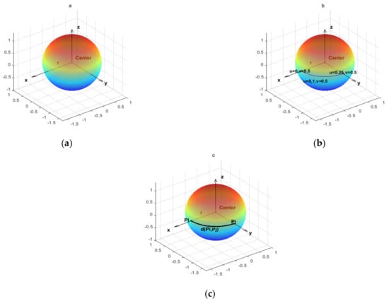
From the perspective of geometry, the center curve can be regarded as a space curve G’ with arc length L. The four basic coordinate systems of the legs are established based on the smooth curve G’, as shown in Figure 2.The P-NBT coordinate system is called the Frenet coordinate system. The T-axis is the tangent vector of the rod’s center curve G’ at point P, which is defined as Equation (1). The N-axis is the normal vector of the center curve G’ at point P, as defined in Equation (2). Axis B is the binormal vector of G’ at point P, which is defined as Equation (3). The three coordinate axes N, B, and T are pairwise orthogonal. At point P, the close plane of the point is determined by the T axis and N axis. The plane defined by N and B is called the normal plane. The curvature and torsion of the curve can completely determine its spatial orientation [22]. Consider an arc of length ds between two points P and P’ on the space curve G’, as shown in Figure 3, Let dϕ be the angle subtended by ds at the center of a circle with radius r. Since ds=rdϕ, the change of the tangent vector with ds is approximately the same with the change of dϕ. As a result, the curvature κ of a space curve is defined by Equation (4).

κ(s)=limΔs→0|ΔϕΔs|=limΔs→0|ΔTΔs|=|dTds|=dϕds

(4)

τ is the torsion of the curve which could be calculated by Equation (5). While the curvature κ is a measure of the deviation of the curve from a straight line, the torsion τ is a measure of the twisting of the curve out of the osculating plane.

The Darboux vector ωF is defined as Equation (6), whose physical meaning is the angular rotation velocity of the Frenet coordinate system (p-NBT) relative to the inertial coordinate system (o-ξηζ) when point P moves along the center curve G’ in the positive direction of the arc coordinate s with unit velocity. The variation of vectors N, B and T can be determined by Darboux vector ωF. Given curvature κ(s) and torsion τ(s), the variation of each coordinate axis vector of Frenet coordinate system (p-NBT) with arc coordinates s can be solved according to Equation (7), and then the shape of the curve can be obtained by Equation (1), as shown in Equation (8). Curvature κ and torsion τ are two independent variables to determine the shape of a space curve, so the degree-of-freedom of space curve is 2.

{dNds=ωF×N=τ(s)B−κ(s)TdBds=ωF×B=−τ(s)NdTds=ωF×T=κ(s)N

(7)

r(s)=∫0sT(σ)dσ+r(0)

(8)

After determining the center curve, the orientation of the cross-section of the rod is further determined to obtain the spatial shape of the rod. The rod is jointly determined by the orientation of its center curve and cross-section. After the center curve of the rod is determined, only the torsion angle of the cross-section needs to be obtained, as shown in Figure 2. Therefore, each rod has 3 degrees of freedom.ω is defined as the angular velocity related to the torsional deformation of the rod, as shown in Equation (9). Its physical meaning is the angular velocity of the cross-section rotation relative to the inertial coordinate system (o-ξηζ) when the point P on the center curve G ‘of the rod moves in the forward direction with unit velocity. where, χ is the angular and (dχds)z is the relative angular velocity of the section with respect to the Frenet coordinate system (P-NBT), and z is the tangent of the center curve. ωF is the relative angular velocity of the coordinate system (P-NBT) with respect to (O-ξηζ). The projected component of the angular velocity ω on the axis of the coordinate system (P-XYZ) on the cross-section is shown in Equation (10).

ωx=κsinχ,ωy=κcosχ,ωz=τ+dχds

(10)

Thus, the shape of the rod can be expressed by three independent variables ωx, ωy and ωz.

Similar to Equation (7). The variation of the coordinate system (P-XYZ) with the arc coordinate s can be described by the ω(s), as shown in Equation (11).

(dxds,dyds,dzds)=(ω×x,ω×y,ω×z)

(11)

2.2. Static Equilibrium of Flexible RodFor the flexible rod, it is divided into micro segments, and each micro segment is analyzed by equilibrium analysis. As shown in Figure 4, P1 and P2 are 2 infinitely closed points on the rod. The reference position vector of origin point O of the inertial coordinate system are r and r + Δr, respectively, and their relative arc coordinates are s and s + Δs, respectively. The static equilibrium is established by taking the micro-element of the rod as the unit, and the internal forces and internal moments of the external section of P1 point are set as -F and -M, respectively, and the internal forces and internal moments of the external section of P2 point are F+ΔF and M+ΔM, respectively. In the equilibrium state at P1, the resultant force and moment of force or torque are 0, as shown in Equation (12). Taking the derivative of Equation (12) to arc coordinates s and converting it to the coordinate system (P-XYZ):

{dFds+ω×F=0dMds+ω×M+z×F=0

(13)

When there is no original curvature, the moment of micro segment on the rod can be expressed through ω as:

Mx=Aωx,My=Bωy,Mz=C(ωz−ωz0)

(14)

where A and B are the flexural stiffness of the rod section around the X-axis and Y-axis, respectively, C is the torsional stiffness of the rod section around the Z-axis. They could be obtained:

A=EIx, B=EIy, C=GIZ

(15)

In Equation (15),

Ix: The moment of inertia of the cross-section with respect to the x axis, Ix=πd4/64.

Iy: The moment of inertia of the cross-section with respect to the y axis, Iy=πd4/64.

Iz: The moment of inertia of the cross-section with respect to the z axis, Iz=πd4/32.

E: Young’s modulus.

G: Shear modulus G = E/(2 + 2μ).

μ: Poisson ratio

d: Diameter of cross section of rod

Equation (12) projected to the coordinate system (P-XYZ) can be transformed into:

{dFxds+ωyFz−ωzFy=0dFyds+ωzFx−ωxFz=0dFzds+ωxFy−ωyFx=0

(16)

{Adωxds+(C−B)ωyωz−Cωz0ωy−Fy=0Bdωxds+(A−C)ωzωx+Cωz0ωx+Fx=0Cdωzds+(B−A)ωxωy=0

(17)

Equations (16) and (17) are static balance equations of the flexible rod. It contains six variables Fx, Fy, Fz and ωx, ωy, ωz. Given the initial condition of the ordinary differential equations, the shape of the rod can be obtained. After the variation of Fx, Fy, Fz and ωx, ωy, ωz with arc coordinate s are obtained, the variation of curvature κ, torsion τ, and torsion Angle χ with arc coordinates s could be solved by Equation (10). By Equation (11), it is transformed into the variation of the axis of the coordinate system (P-XYZ) with arc coordinate s.