Introduction

Formoterol is a rapid-onset, long-acting β2 agonist, typically administered by inhalation in combination with low-to-high doses of corticosteroids for control-based asthma management in asthmatic patients [Global Strategy for Asthma Management and Prevention—GINA—2022 update (Ginasthma, 2022)]. Formoterol is also used as reliever medication in association with low dose corticosteroids. In fact, different studies have demonstrated that it is effective as short-acting β2 agonists providing rapid bronchodilation within 1–3 min of administration and that its duration of action extends to up to 12 h after inhalation (Hekking et al., 1990; Palmqvist et al., 1997; Ringdal et al., 1998; Seberova and Andersson, 2000; Welsh and Ctes, 2010). Moreover, results from previous studies (Castle et al., 1993; Nelson et al., 2006) provide support to its use in combination with inhaled corticosteroids (ICSs) and demonstrate its greater effectiveness in comparison with salmeterol. Other studies (Faulds et al., 1991; Politiek et al., 1999) compare the efficacy of formoterol against both short- and long-acting β2 agonists, concluding that formoterol and salbutamol have roughly the same efficacy.

The Aerolizer®, a dry powder inhaler (DPI), has been introduced for use for the administration of formoterol instead of the traditional metered-dose inhalers (MDI), which deliver a formoterol solution aerosol. DPIs are particularly useful for patients with difficult coordination in inspiration and assure the correct pharmacological dose administration in these patients.

Several studies prove the efficacy and safety of formoterol delivered via Aerolizer (Bensch et al., 2001; Pleskow et al., 2003), when compared with albuterol via Metered Dose Inhaler. Moreover, formoterol DPI provides an equivalent bronchodilating effect with respect to formoterol MDI in asthmatic patients (Bousquet et al., 2005).

In a previous work Gaz et al. (2012), a mathematical approach to the description of the fate of a compound administered by the inhalation of an aerosolized cloud of droplets was presented. In that (pharmacokinetic/pharmacodynamic—PK/PD) model the relevant pharmacokinetics was represented with the use of five compartments. Two of them were aggregated compartments representing the bronchial tree and associated muscle divided in turn into sub-compartments representing the spatial dimension along the depth of the bronchial tree. The model proposed in that work differs from traditional PK/PD models by introducing a simplified geometrical and functional description of the bronchial tree, leading to the direct computation of the approximate airflow. Anatomical and geometrical features, such as bronchial branching and smooth muscle distribution, are taken into account.

This approach takes a middle road between pure compartmental modeling of the respiratory system, along with the blood-to-tissue distribution of substances (giving rise to a system of nonlinear ordinary differential equations, ODE’s), and full Computational Fluid Dynamics (CFD) (Donovan et al., 2012; Vos et al., 2013; De Backer et al., 2015), in which the respiratory system of a given subject is geometrically modeled in three-dimensional space, typically on the basis of CT scans or other medical images.

In this simplified geometry approach (Gaz et al., 2012), modeling of the bronchial region takes into account a partial differential process in one spatial variable, because many crucial PK and PD features depend on the depth into the bronchial tree. The distribution of anatomical and physiological characteristics down the bronchial tree can thus be taken into account in order to obtain a physiologically-based representation of the pharmacodynamics effect of inhaled bronchodilators.

The simulations obtained with the simplified geometry model agreed very well with expected behavior of the time-course of forced expiratory volume in the first second (FEV1) after the administration of inhaled medication. The main advantage of the new model with respect to standard PK/PD formulations was thought to be in the closer mechanistic approximation to the actual physiology of respiration and to the corresponding drug particle deposition, whereas its main advantage with respect to full-blown Computational Fluid Dynamics was the possibility of representing many subjects within the limits of a reasonable computational burden.

The aim of the present study is therefore that of validating the simplified geometry modeling approach against clinical efficacy data. In order to do so, we will proceed to build a Clinical Trial Simulation. The reasoning proceeds in three steps: a simulated population reflecting the demographics and the disease–related characteristics of Pleskow’s study population (Pleskow et al., 2003) is created (The Simulation step); a modified version of the simplified geometry PK/PD model (Gaz et al., 2012) is used to compute airflow response to treatment for each single virtual patient (The Modelling step); the FEV1 results obtained in virtual samples are compared with those obtained in the real sample of adolescent and adult asthmatics studied by Pleskow et al. (2003) in order to validate the model in its new formulation (The Parameter Estimation step).

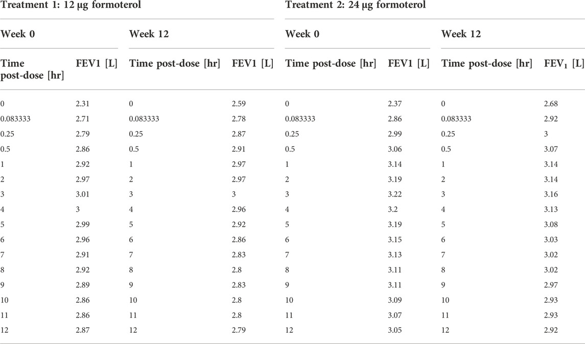
MethodsPleskow’s study design

Pleskow’s study (Pleskow et al., 2003) was a multicenter, randomized, double-blind, double dummy, parallel-group study. The aim of the study was that of comparing efficacy and tolerability of twice-daily formoterol dry powder 12 μg and 24 μg (Foradil) delivered via Aerolizer inhaler against four times daily albuterol (salbutamol) 180 μg delivered via metered dose inhaler (MDI). A matching placebo group was also used for comparison. Adolescent and adult patients with mild-to-moderate asthma were screened and followed for a run-in period before being randomized to one of the above four treatment groups. The double-blind treatment period lasted 12-week. The design of the study contemplated a spirometry evaluation, consisting of FEV1, Forced Vital Capacity (FVC) and maximum mid-expiratory flow (FEF25–75%) evaluated at 0, 5, 15, and 30 min and hourly from 1 to 12 h—post-dose—at weeks 0, 4, 8, 12 and at the final visit. The primary efficacy end-point of the study was the serial FEV1 values over the 12-week study (from week 0 to week 12). The measurements of FEV1 over the 12 h, at week 0 and week 12, are related to the post treatment administration period (post-dose).

Results from the study showed that FEV1 measurements from the formoterol treatment groups were clinically and statistically higher than those from the placebo group. For more details of this study refer to Pleskow et al. (2003).

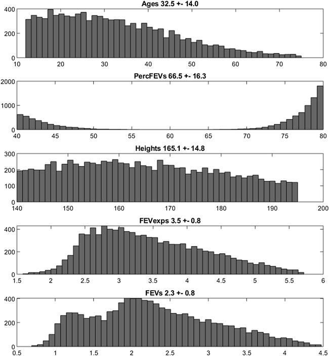
The Simulation step: Reproducing the target population characteristics

The first objective of the present work was that of virtually reproducing Pleskow’s populations in terms of both demographic and disease-associated characteristics. In the present work only the groups undergoing treatment with formoterol (12 μg or 24 μg) were considered. The demographic covariates taken into account were age, gender and height; the covariates associated with the disease severity were expected FEV1, as function of the above demographic characteristics according to the Quanjer GLI-2012 regression equations (Quanjer et al., 2012), as well as fraction of predicted FEV1. Reference mean and standard deviation values for the above variables measured at baseline, were taken from Table 1 of Pleskow et al. (2003). 10,000 virtual patients were generated so as to obtain age, FEV1, percentages of predicted FEV1 and gender distributions as close as possible (in terms of averages and standard deviations) to those observed in Pleskow’s patient sample. The covariate distributions were simulated under parametric assumptions as follows. For age, a truncated normal distribution was adopted. A bi-modal normal distribution was used to generate the percentage of predicted FEV1 with most of the subjects near the 40% or the 80% limits and few subjects in between: the presence of two subpopulations was therefore hypothesized, one presenting with a low degree of basal obstruction and one presenting with a more severe air obstruction (this was necessary in order to match the observed sample characteristics). Even if such a distribution could in principle appear to be little plausible, however there is no unimodal probability distribution able to reproduce the observed Pleskow’s data: patients within a narrow range of percentage of predicted FEV1 (from 40% to 80%), with an average value of 66.5 and a quite large standard deviation of 16.3%. Males and females were generated in the same proportions as reported by Pleskow, while the distribution of FEV1 was generated from the distributions of the expected FEV1 (ExpectedFEV1) and of the percentage of predicted FEV1 (PercFEV1) according to the formula:

FEV1=ExpectedFEV1×PercFEV1100

The above computation refers to the baseline condition, that is before the administration of formoterol.

Because Table 1 in Pleskow et al. (2003) did not report population averages and standard deviations of heights in females and males (height being a necessary predictor for the computation of the expected FEV1), these values, for the two populations, were found by minimizing, with respect to θ, the following loss function:

Lθ=TargetMeanFEV1−MeanFEV1θMeanFEV1θ2+TargetStDevFEV1−StDevFEV1θStDevFEV1θ2

where θ is the parameter vector containing the generating population height and standard deviation parameters for males and females. These parameters were used to sample the heights from two normal distributions, one for females and one for males. Once the gender was generated according to the Pleskow’s gender distribution, height was sampled with one or the other distribution according to the generated gender. In the above loss function TargetMeanFEV1 and TargetStDevFEV1 are the mean and standard deviation, respectively, of the observed mean and standard deviation reported for the Pleskow’s sample. MeanFEV1(θ) and StDevFEV1(θ) are functions of θ by means of the variable ExpectedFEV1 which depends indeed on the height. The optimization procedure was started with different values of mean and standard deviation for males and females: 170 ± 27 and 160 ± 22 cm, respectively.

Notice that truncated distributions were used because the originally enrolled patient samples were confined to given age and fractional expected FEV1 brackets.

Table 1 reports the average values and standard deviations (or percentages as appropriate) of the observed (from Pleskow’s patient sample) and simulated (virtual subjects from the simulation step) demographic and disease-related variables. Table 2 reports the average observed FEV1 at post-dose times both at week 0 and week 12.

TABLE 1. Baseline Pleskow’s population characteristics along with the obtained average characteristics from the two simulated populations (10,000 patients each).

TABLE 2. Pleskow’s post-dose observed FEV1 on the first day (week 0) and at week 12 of double-blind treatment with formoterol 12 μg or 24 μg delivered via Aerolizer.

The Modelling step: A mixed compartmental and distributed PK/PD modelThe pharmacokinetics equations

In Gaz et al. (2012) a mixed compartmental and distributed PK/PD model was proposed, where the pharmacodynamic effect was derived from the (distributed) concentrations of drug in the effect compartment (bronchial muscle). The model equations are reported below:

dPtdt=−kxp+kmpPt−kgpPt+kpgGt+kpm∫z0zmaxMz,tdzVdistrW,P0=0(1)dGtdt=−kpgGt−kxgGt+kgpPtVdistrW,G0=η1−ρbgD0(2)dBz,tdt=−kmbBz,t+kbmMz,t+φw∂2Bz,t∂2z2, Bz,0=fzηρbbD0(3)dMz,tdt=−kpm+kbmMz,t+kmbBz,t+kmp∫dzPt⋅VdistrW, Mz,0=0∀z∈zmin,zmax(4)dUtdt=ψ kxpPt VdistrW, U0=0(5)

The above model formulation hypothesizes that the sprayed dose D0 is split into two parts, one being the amount actually delivered to the mouth ηD0, and the other one (1-η)D0 being the fraction of the active compound dose D0 remaining in the device itself. A fraction ρbb (where bb is the drug’s bronchial bioavailability) of the delivered dose reaches the spatially distributed compartment B (Eq. 3), spreads instantaneously over the entire bronchial tree according to a probability density f(z), and is transferred to the bronchial muscle fibres (spatially distributed compartment M, Eq. 4) with apparent first order transfer rate kmb. The remaining fraction (1-ρ)η bgD0 of the delivered drug is transferred to the bioavailable gastrointestinal drug depot G (Eq. 2), where bg is the gastrointestinal drug bioavailability.

The probability density f(z), appearing in the boundary condition of Eq. 3, depends on the physical characteristics (aero and hydrodynamics) of the aerosolized particles. The symbol z represents the single spatial dimension, expressed as a standardized distance of a point along the bronchial tree from the end of the larynx. The probability density of deposition f depends therefore on z. After its deposition, the compound diffuses in time along the bronchial tree with a diffusion coefficient φw and is locally absorbed from the mucosa into the bronchial muscle compartment.

The compound is then transferred from compartments G and M into the plasma compartment P (Eq. 1) with apparent first order transfer rates kpg and kpm. From plasma, the drug is eliminated at a rate kxp into the compartment U (Eq. 5), representing the quantity of formoterol in the urine, with ψ indicating the recovery fraction of the drug. The parameter kgp represents hepato-biliary extraction whereas the parameter kxg represents partial gastrointestinal elimination: in the present simulation both are set to zero. Moreover, given the small amount of drug actually transferred to bronchial smooth muscle and the relatively good blood perfusion of the muscle itself, the parameter kbm was also set to zero. Finally, although the model allows bidirectional compound exchange between the P and M compartments, so that available drug could in principle be transferred from plasma to bronchial muscle, also the parameter kmp was set to 0, reflecting the very minor role of back-transfer of active substance from plasma to the effect site.

The pharmacodynamics equations

All the hypotheses on which the mathematical representation of the geometrical and behavioural features of the bronchial system is based upon are detailed in Gaz et al. (2012). The key assumptions are that bronchioles at the same relative distance down the bronchial tree present the same structural features and behaviour and that the drug effect on a subject depends on the position, along the bronchial tree, where the compound is deposited (Gaz et al., 2012). Briefly, at the bronchial level, β2-adrenergic receptors, when stimulated by the presence of the drug, determine local bronchodilatation: the diameters of the bronchioles increase with a resulting decrease of airway resistances (to which airflow is inversely related by the first Ohm’s law). The model describes the direct computation of the approximate Forced Expiratory Volume in 1 s (FEV1), as the volume moved in 1 s under constant expiratory pressure, assuming constant bronchial geometry and elastic recoil, given the PK of the substance.

We report below the main equations and modelling assumptions.

Let δm(z,0) be the bronchial profile at time 0 representing the degree of patency of the airways, expressed as fraction of normal bronchial diameter at each z. For a healthy subject, the disease profile is identically equal to 1; in case of a broncho-constricted subject, as for example in an asthmatic subject, the constriction profile has been represented by

δmz,0=1−Ae−z−b22c2(6)

where A is the maximal restriction amplitude (as a fraction of 1), b is the position of the maximal bronchial restriction along z and c is the standard deviation of the Gaussian curve which determines the width of the constriction. In the original work (Gaz et al., 2012), the drug dynamic effect over time was associated with the bronchial muscle content of the active principle as follows:

dδmz,tdt=kmorδmz,0−δmz,t+kmedhzMz,t1−δmz,t(7)

where the initial condition in the above equation is the disease profile described in Eq. 6; M(z,t) is the drug content density of bronchial muscle at time t and position z, as computed from the kinetic part of the model (Eq. 4); kmor is a constant representing the degree of the subject’s morbidity (as the rate of spontaneous return of the bronchial diameter towards its diseased profile), while kmed represents the medicinal efficacy of the drug (as the rate of modification of the bronchial profile towards unity, or towards 100% patency).

In the present formulation, instead, in order to reproduce the observed initial fast rise and subsequent progressive further rise followed by gradual fall of the observed effect, a modification of Eq. 7 proved necessary: while in Eq. 7 the compound passes directly from the bronchial mucosa into the muscle compartment effect site, here it is hypothesized that two parallel delay compartments (one faster and one slower) have to be interposed between the mucosa and the muscle compartment:

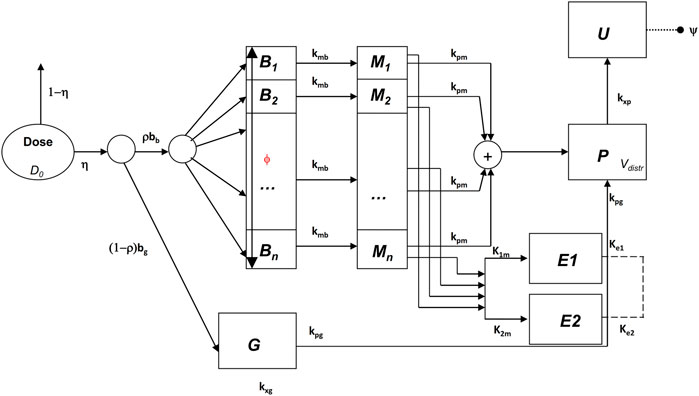
dδmz,tdt=kmor⁡exp⁡(−λ1E(z,t))δmz,0−δmz,t+kmedhzhmax(1−exp⁡(−λ2E(z,t))1−δmz,t(8)dE1z,tdt=k1mMz,t−ke1E1z,t,E1z,0=0∀z∈zmin,zmax(9)dE2z,tdt=k2mMz,t−ke2E2z,t,E2z,0=0∀z∈zmin,zmax(10)dEz,tdt=ke1E1z,t+ke2E2z,t−kxeEz,t,Ez,0=0∀z∈zmin,zmax(11)

The drug dynamic effect over time is associated with the activity of the compound at a distal site E (which could represent the turnover rate of calcium ions in the sarcoplasmic reticulum), affected possibly by concurrent, parallel slow and fast delay mechanisms E1 and E2. See Figure 1 for a graphical representation.

FIGURE 1. Schematic representation of the pharmacokinetic/pharmacodynamic model.

The function h(z) in Eq. 7, as well as in Eq. 8, represents the β2-adrenergic receptor density, which, in the present formulation, is hypothesized to vary along the bronchi in an approximately linear fashion:

where hmin is the value of the receptor density at z = 0, and αh is the approximately linear increase in receptor density per cm. The simpler (linear) formulation (Eq. 12) of the increasing receptor density down the bronchial depth resulted in any case numerically very similar to the original (Gaz et al., 2012) nonlinear formulation (Hill function). Again, the first term on the right-hand side of Eq. 8 represents the natural tendency of the disease condition to constrict bronchi towards the untreated state: its size depends on the effect entity as well as on the achieved level of broncho-dilatation. The second term on the right-hand side of Eq. 8 is 0 until the drug is administered [since E(z,0) = 0], then, as soon as the drug reaches the bronchial mucosa, the compound passes into the delay compartments and thence reaches the effect site.

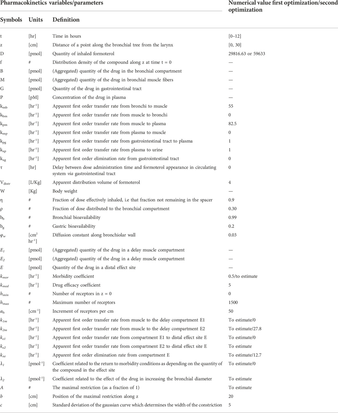
All state variables and model parameters of the pharmacokinetic equations as well as of the pharmacodynamic equations are described in Table 3. Figure 1 reports the schematic diagram of the PK/PD model.

TABLE 3. Model pharmacokinetics and pharmacodynamics variables and parameters.

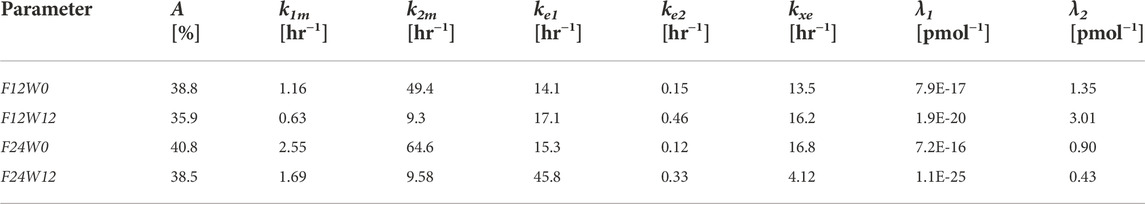
The parameter estimation step

Due to evident a-priori unidentifiability, several parameters were kept fixed throughout the optimization process. Fixed model parameters were set to the original values used in Gaz et al. (Gaz et al., 2012) and are reported in Table 3. The free parameters to be estimated are related only to the pharmacodynamic part of the model and were fitted to the four sets (formoterol 12 μg at week 0, F12W0, and at week 12, F12W12; formoterol 24 μg at week 0, F24W0, and at week 12, F24W12) of experimental post-dose FEV1 observations over time derived during the visit after the inhalation of a single dose of formoterol and obtained by Figures 1, 2 of Pleskow et al. (2003) where the mean FEV1 values on the first (week 0) and last day (week 12) of the two treatment regimens (F12W0, F12W12, F24W0 and F24W12) are shown. Reliable values of the coordinates of the points were retrieved by using the software Plot Digitizer (https://plotdigitizer.com/app).

Initially, the parameter estimation process involved 8 of the pharmacodynamics parameters, whose estimates are reported in Table 4 (A, k1m, k2m, ke1, ke2, kxe, λ1, λ2). A Nelder-Mead simplex direct search was used for all optimizations and a weighted least squares estimation approach was followed. The precision of the estimates was computed by the asymptotic approximation:

where

σ2=1n−py−y^ TWy−y^

n and p are the total number of observations and the number of the free parameters, respectively, J is the Jacobian matrix with element (i,j) equal to ∂yi,jθ∂θ and where W is the diagonal matrix of weights whose elements are the inverse of the squared of the expectation.

TABLE 4. Estimates of the Model free parameters at the beginning (week 0) and at the end of the study (week 12) for the two treatment regimens, from the first optimization process.

Since not all parameters could be estimated with precision (invertibility problems of the variance and covariance matrix at the optimum) the model was simplified by eliminating the slow delay mechanism E1. With the elimination of compartment E1, parameters λ1, k1m, ke1 also were discarded. The parameter kmor, representing the degree of morbidity, was allowed to vary and parameters k2m and kxe were set to the average values obtained in the previous fittings. In total, this second step required therefore the estimation of only four parameters: A, kmor, ke2 and λ2.

All computations were performed with the R2011b version of Matlab.

FEV1 trend over time for the simulated populations

For each subject in the four simulated populations, the FEV1 trend over time (from time 0–12 h) was simulated according to the PK/PD model described above.

The parameter A in Eq. 6, representing the maximal restriction, is one of the model parameters to be estimated from Pleskow’s observations. For each simulated subject, however, it can be computed in percentage terms directly from the computed percentage of predicted FEV1 value (PercFEV1(s), where s indicates the simulated subject), made available from the Simulation step as described above.

The reasoning and the assumptions are as follows: let a bronchial section in normal conditions be approximated by a circumference with diameter equal to 1. Under a restriction (expressed in terms of percentage) of width RestrPerc the useful surface becomes:

where p is a parameter that translates the functional restriction in geometrical bronchial diameter reduction, and k is a constant value representing the total number of available surfaces along the bronchial tree (Gaz et al., 2012).

Since FEV1 can be computed directly as the product between the pressure delta and the useful surface, for a normal subject (under healthy conditions) the approximated expected FEV1 is:

where ΔP is the pressure delta; the percentage of predicted FEV1 (given by the percent ratio between the actual FEV1, FEV1restr and the expected FEV1, FEV1norm) for the subject s is therefore:

PercFEV1s=FEV1restrFEV1norm×100=ΔP×kπ1−p×As22ΔP×kπ122×100=1−p×As2×100(15)

from where the dependency on ΔP and k vanished, and from which it follows that:

As=1−PercFEV1s/100p(16)

The unknown parameter p can be determined minimizing the following loss function:

p^=minpAF24W0¯p−A^F24W02(17)

where AF12W0¯ and AF24W0¯ are the averages of A(s) computed for the 10,000 simulated subjects in the F12W0 population and for the 10,000 simulated subjects in the F24W0 population respectively according to Eq. 16, and where A^F12W0 and A^F24W0 are the estimates of parameter A in Eq. 6 obtained by fitting the model onto the datasets F12W0 and F24W0 respectively with the first optimization step.

The function A(s) for the two populations at week 12 (populations F12W12 and F24W12) can be computed hypothesizing that the percentage of predicted FEV1 for the two simulated populations is different at week 12 with respect to week 0 due to an additive factor Δ (with Δ ≥ 0) expressing the effect of treatment during the course of the study period. The parameter Δ is determined, with p fixed at the estimated value p^, by minimizing the following expression:

Δ^=minΔ+AF24W12¯PercFEV1,F24W12Δ,p^−A^F24W122.(18)

Once having obtained for each simulated subject his/her own percentage restriction, other model parameters were set to the specific value for the subject when available (age, gender, height, expected FEV1). The remaining parameters were set to the estimated values from the Parameter Estimation step or were kept fixed to their original values as reported in Table 1. Eqs 17, 18 proved necessary in order to estimate the Pleskow’s populations features in terms of percentage of restriction. In an actual clinical setting, the patients might be undergone a sequence of spirometry tests after drug administration, and the model can be fitted to the patient’s observed data for estimating the parameter A, which indeed represents the degree of bronchial restriction.

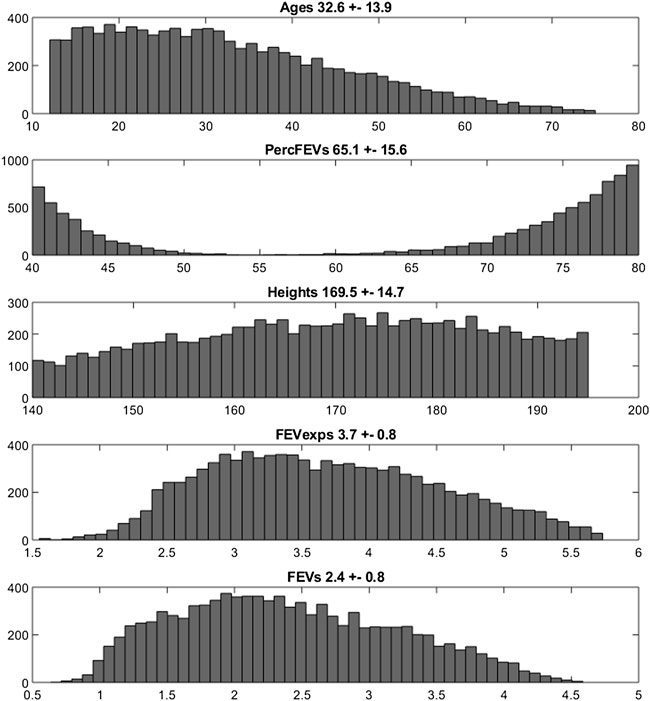
Results

The empirical distributions of the demographic and disease-related characteristic (age, height, expected FEV1, observed FEV1 and percentage of predicted FEV1) of the two simulated populations are shown in Figures 2, 3 (formoterol 12 and 24 μg, respectively). Average heights and the relative standard deviations were estimated to be 165.1 ± 14.8 and 169.5 ± 14.7 cm for 12 and 24 μg formoterol treatment. The values in the two gender subsamples resulted to be 169.2 ± 15 cm and 161.1 ± 13.5 cm for males and females, respectively, in the 12 μg formoterol population. Values for males and females in the 24 μg formoterol population were 172.5 ± 14.5 and 165.7 ± 14.1 cm, respectively. The obtained values approximate the average gender-specific height in North and Central America, where the study is supposed to have been conducted: 173 cm and 160 cm for males and females, respectively (https://www.worlddata.info/average-bodyheight.php). Note that there is a difference between the average heights obtained in the 12 μg and 24 μg formoterol populations: the mean heights are lower in the lower-dosed population. Since population heights were not reported in Pleskov’s work, it is not possible to say whether the simulated populations closely resemble the original populations in terms of heights; however, the difference could be due to the fact that a lower dose was mainly given to younger individuals.

FIGURE 2. Histograms of frequencies of the simulated demographic and related-disease characteristics for the population undergoing 12 μg of formoterol via Aerolizer.

FIGURE 3. Histograms of frequencies of the simulated demographic and related-disease characteristics for the population undergoing 24 µg of formoterol via Aerolizer.

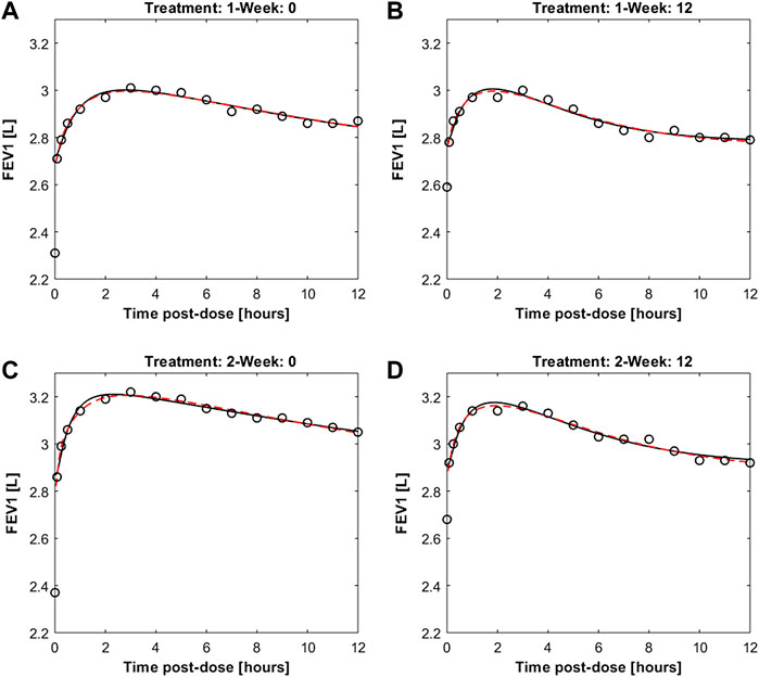
Figure 4 reports the observed and predicted post-dose values of FEV1 over time in the two treatment regimens at week 0 and at the end of the study period for both the two fitting procedures. The dashed red lines are the predictions obtained estimating the eight pharmacodynamics parameters; continuous black lines represent the predictions obtained with only four free parameters. Panels A and B report the expected responses for treatment formoterol 12 μg at week 0 and at week 12 respectively; panels C and D report results related to treatment group formoterol 24 μg. The estimates of the model free parameters obtained in the two optimization procedures are reported in Tables 4, 5.

FIGURE 4. Panels (A,B) report observed and predicted mean FEV1 on the first day and at week 12 of double-blind treatment with formoterol 12 μg delivered via Aerolizer respectively; panels (C,D) report instead observed and predicted mean FEV1 on first day and at week 12 of double-blind treatment with formoterol 24 μg respectively.

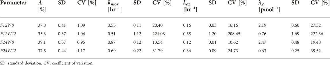
TABLE 5. Estimates of the Model free parameters along with the respective standard deviations and coefficients of variation, at the beginning (week 0) and at the end (week 12) of the study for the two treatment regimens, from the second optimization process.

From Table 4 the four estimates of restriction were used to estimate once the parameters p and Δ from Eqs. 17, 18, useful for the computation of the percentage of restriction for each individual of the simulated populations. Table 5 reports the final estimates of the free model parameters when only four parameters were allowed to vary. The estimates of the restrictions continue to be coherent with the mean values obtained from the 10,000 simulated subjects of the two populations as described in the subsection “FEV1trend over time of the simulated populations” above. For formoterol 12 μg the estimates were 37.8% and 35.3% at the beginning and at the end of the study period, respectively versus the average values over the 10,000 subjects of 39.0% at week 0 and 36.4% at week 12. For formoterol 24 μg the estimated values were 39.1% and 37.5% whereas the computed averages were 40.6% and 38.0%.

All free parameters were identifiable in all experimental situations, with the exception of the 12 μg experimental regime at week 12, where the Coefficient of Variations (CVs) resulted to be larger than 200% for all the free parameters except for parameter A (percentage of restriction). Conversely, in the F12W0, F24W0 and F24W12 experimental situations CVs varied from a minimum of 0.96% to a maximum of 39.5%.

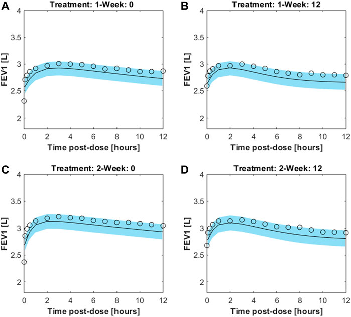
The trend over time of FEV1 after drug administration was simulated for 200 sets of 100 individuals each. The individual trend was obtained by running the model with parameters set to the fixed and estimated values from the second optimization procedure, except for some specific individual parameters (age, height and gender, useful for the computation of the expected FEV1; percentage of restriction). For each set the average trend was computed along with its 2.5% and 97.5% percentiles. Figure 5 shows the mean FEV1 trends over time (black lines) from the 200 sets, as well as the 95% confidence bands of means for the simulated populations for the two experimental regimes both at week 0 and at week 12; Pleskow’s observations (circles) are also reported.

FIGURE 5. Results from 200sets of 100simulated individuals, each. For each simulated individual, trend over time of FEV1 was simulated by running the model with parameters set to the fixed and estimated values from the second fitting procedure, except for the specific individual parameters age, height, gender and percentage of restriction. Continuous black lines are the mean trends over time from the 200sets whereas light-blue areas represent the 95% confidence bands of means (between its 2.5% and 97.5% percentiles). Results are showed for the two experimental regimes both at week 0 and at week 12 for double-blind treatment with formoterol 12g [panels (A,B), respectively] and with formoterol 24g [panels (C,D), respectively].The image used in Figures 5 and 6 have part labels AD; however, the description is missing in the caption. Could you clarify this? Provide revised files if necessary.

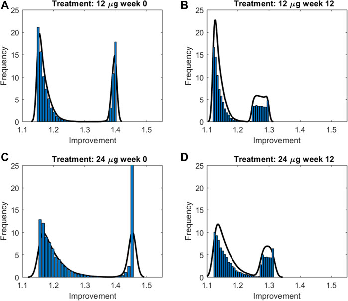
In order to summarize the efficacy of treatment, for each simulated subject an “Index of Improvement” was computed as the ratio between the average predicted FEV1 over time and the basal FEV1 level. Figure 6 reports the frequency distributions of the index along with the relative kernel density estimation of the distributions. All the distributions show a bimodal shape, in all likelihood reflecting the hypothesized bimodal distribution of asthma severity. As an example, let consider the 24 μg formoterol population at week 0 (panel A) and divide the population into two subpopulations: individuals who show a large improvement (larger than 1.35) and individuals with a small improvement (smaller than 1.3). The analysis of the characteristics of the individuals belonging to the two different distributions showed that the two subpopulations do not differ significantly with respect to distribution of gender, height, age and hence expected FEV1 (males: 55.9% vs. 55.8%, height: 169.5 cm vs. 169.6 cm; age: 32.9 years vs. 32.4 years; expected FEV1: 3.7 L vs. 3.7 L in the group with large and small improvement, respectively) whereas the two subgroups show a very different baseline FEV1 expressed as percentage of predicted FEV1: 44.9 ± 2.5% vs. 77.5 ± 3.9% in the subpopulation with large improvement and in the subpopulation with small improvement, respectively, which translates into a larger percentage maximal restriction: 67.2 ± 3.7% vs. 24.4 ± 4.6%, respectively.

FIGURE 6. Frequency distributions along with the relative kernel density estimation of the improvement indices computed for the two treatment groups at week 0 and 12 for double-blind treatment with formoterol 12g [panels (A,B), respectively] and with formoterol 24;g [panels (C,D), respectively].

Figure 7 reports instead the Improvement index as a function of percentage of predicted FEV1 for a male subject, 175 cm height, aged 30 years, undergoing 12 μg (dotted lines) or 24 μg (continuous lines) of inhaled formoterol at week 0 (red lines) and week 12 (blue lines). As expected, the Improvement decreases with increasing percentage of predicted FEV1, highlighting a larger effect of treatment both in the presence of worse conditions and at the beginning of the experimental period.