, k ∈ , i ∈ continuity constraints, the displacement, velocity, acceleration, jerk, and snap at the track point should also be continuous. That is satisfied fμ(k)(Ti)=dik, where μ ∈ , k ∈ , i ∈ . It can be written as an equality constraint.

We need to fix each trajectory time Tj = 0.1s for all joints. Ensure that all robot joints reach the desired angle and end position at the same moment is always stable.

Summarizing the above constraints and cost functions, they are written in matrix form.

• Desired angle constraint:

fj(k)(Tj)=xj(k)    (63) ⇒∑i≥ki!(i-k)!Tji-kpj,i=xT,j(k)    (64) ⇒[...⋯ i!(i-k)!Tji-k⋯ ...][:pj,i:]=xT,j(k)    (65) ⇒[i!(i-k)!Tj-1i-k::i!(i-k)!Tji-k][:pj,i:]=[x0,j(k)xT,j(k)]    (66)

• Continuity constraint: smoothness constraint ensures continuity between trajectory segments without giving a specific derivative.

fj(k)(Tj)=fj+1(k)(Tj)    (68) ⇒∑i≥ki!(i-k)!Tji-kpj,i-∑l≥kl!(l-k)!Tjl-kpj+1,l=0    (69) ⇒[⋯ i!(i-k)!Tji-k ... ... -l!(l-k)!Tjl-k ⋯]       [pj,i::pj+1,l]=0    (70) ⇒[Aj-Aj+1][pjpj+1]=0    (71)

Substitution function:

J(T)=∫Tj-1Tj(f4(t))2dt=[:pi:]T[…i(i-1)(i-2)(i-3)l(l-1)(l-2)(l-3)i+l-7Ti+l-7…][:pl:]    (72) Jj(T)=pjTQjpj    (73)

Writing the above problem as an equation constraint in standard form, then the quadratic programming problem can be expressed as:

min[p1:pM]T[Q1000:000QM][p1:pM]    (74) s.t. Aeq[p1:pM]=deq    (75)

The above equation is a linear constraint quadratic programming problem (QP).

Collision avoidance

UVMS requires only six degrees of freedom to reach an arbitrary position in underwater motion. Adding a manipulator gives the entire system more than six degrees of freedom, resulting in the redundancy of degrees of freedom. Kinematic redundancy allows the planner to satisfy additional constraints, such as collision avoidance. Researchers have mainly focused on approximating the robot or the obstacle with strictly convex targets and considering only the closest points in the detection algorithm to avoid collisions to reduce computational effort.

The optimization process has no environmental constraints after the trajectory planning solution based on the minimum snap principle. When a new trajectory is encountered after optimization, the obstacles force the trajectory to be modified again, wasting computational resources and reducing the planning frequency. For example, it is necessary to add constraints on the environment during optimization, generally based on hard constraint solving. The hard constraint solution is to generate a safe region in the environment by extending the algorithm and using it as a hard constraint. Adding hard constraints in the optimization process forms a convex polygon, which transforms the QP problem into a convex optimization problem that can be solved by convex optimization algorithms such as the interior point method.

While the process of underwater obstacle avoidance, most of the surrounding objects are non-strictly convex polyhedra, and these approximation methods are not accurate enough when operating in close range. The problems in the practical application process are ignored. Because the remaining safe regions are treated equally during optimization, there is no good way to handle the extreme cases with underwater sensor noise. The optimized trajectory may go past the edge of the safety zone. Once the controller makes an error, it leads to a severe failure of the manipulator body by colliding with the internal and external environment. Inspired by the penalty function, we propose a more intuitive collision-free motion planning method oriented to UVMS.

An improved collision avoidance method based on soft constraint

By design, we use the principle of soft constraint to improve the collision avoidance method. The essence of the soft constraint method is to apply a “pushing force” to push the trajectory away from the direction of the obstacle. The core problem is the designed objective function. When the objective function is not set correctly, the path may hit an obstacle, which is the shortcoming of soft constraint. Therefore, a gradient-based optimization algorithm sets the objective function to impose a soft constraint on the underwater manipulator to push the underwater manipulator body away from the obstacle.

For Equation 16, the objective function becomes:

J=Js+Jc+Jd=λ1J1+λ2J2+λ3J3    (76) JS=∑μ∈∫0T(dkfμ(t)dtk)dt    (77) [dFdP]TCTM-TQM-TC[dFdP]=[dFdP]T[RFFRFPRPFRPP][dFdP]    (78)

where the smoothness cost function Js is the cost of smoothness generated using minimum-snap.

Jc=∫T0TMc(p(t))ds     =∑k=0T|δtc(p(Tk))‖‖v(t)‖‖δt,Tk=T0+kδt    (79)

where the collision cost function Jc, i.e., the collision cost, penalizes obstacles that are too close.

where the kinetic cost function Jd penalizes exceeding the kinetic constraints. Since the objective function of penalizing the velocity and acceleration is not a convex function, it needs to be solved by step-by-step derivation. The smooth term solution is shown in the previous derivation, and the relationship between the collision term and the free variables dpμ is as follows.

Jc=∫δtdpμ},        μ∈    (80)

where the F and G are, respectively:

F=TLdp, G=TVmLdp    (81)

where Ldp is the right half of the matrix M−1C, Vm is the mapping matrix of joint position variables to joint velocity variables, T=[Tk0,Tk1,…,Tkn].

The second-order derivative results in:

Ho=[∂2fo∂dPx2,∂2fo∂dPy2,∂2fo∂dPz2]∂2fo∂dPμ2=∑k=0τ/δtδt    (82) Simulation results

In this section, the task priority processing strategy and soft-constrained trajectory optimization objective designed in this paper are verified on a kinematically redundant underwater vehicle manipulator system. The system consists of a free-floating underwater vehicle and a seven-function manipulator. The simulation is performed in a MATLAB/Simulink environment.

Case 1: Test the given tasks

The simulation phase first initializes the UVMS for safe waypoint navigation. Afterward, we move the vehicle to a position close to the currently defined end-effector target position, slightly above the target position. Finally, the action change is triggered, and the UVMS executes the ocean float operation. We do not consider any disturbances and assume that the robot can provide the desired speed without delays. In addition, once the robot reaches the desired position, the rest of the tasks are responsible for the end-effector reaching the desired target position and orientation, so the “PC” task will also be closed. For the end-effector to operate as a stationary-based robot, we need to constrain the vehicle not to move. Because, as we noticed, the vehicle will “help” the arm to reach the desired position by moving itself (in line with the expected behavior of the tool task). To avoid this problem, we need to perform a non-reactive task to constrain the vehicle to move or reach the operating position where the task will make the vehicle move. In this case, we test UVMS landing on the seafloor, try the vehicle to its target coordinate system, and then use the end-effector to reach the operational target position. Observe whether the vehicle does not move and perform the ocean float operation of the UVMS.

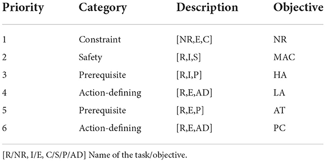
The uniform hierarchy of tasks we use and their priorities, with the addition of constrained tasks at the priority level, is described in Table 3, with non-reactive tasks (“NR”) added at the top of the hierarchy to constrain the vehicle not to move.

Table 3. Control tasks and priorities for fixed base manipulation operations.

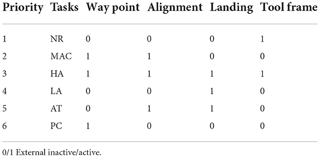
We have the following tasks in an active/inactive state for each of the different phases, is described in Table 4.

Table 4. Examples of external activation states for different tasks.

We conducted a multitask prioritization strategy experiment to explain the task prioritization strategy better. First, multitasking is divided into multiple action phases.

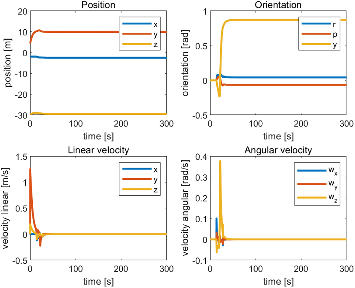
1. Action A, safe waypoint navigation with all the safety tasks enabled. This action finishes when the position error is below a fixed threshold (in this case 0.1 m), as Figure 5 shows.

2. Action B, alignment to the nodule with all the safety tasks enabled. This action finishes when the misalignment error is below a fixed threshold (in this case 0.07 m).

3. Action C, landing, and smooth rotation align with the target. This action finishes when the vehicle touches the seafloor (in the simulation, this happens at approximately 0.17 m).

4. Action D, manipulator actuation after landing. In this action, Vehicle Null Velocity task is enabled, preventing vehicle movements. The only movement will be the extension of the manipulator to reach the desired target position.

Figure 5. Position-directional linear velocity angular velocity tracking curve of the completed vehicle initialization.

From Figure 6, we observe that the position and orientation errors of the vehicle base remain almost constant after 30 s of simulation when the UVMS has completed t