Galileo is a standard GA tailored to deal with combinatorial fragment spaces. It implements classical genetic operators like crossover and mutation in a chemistry-aware fashion such that all molecules created are valid fragment space products. The GA can be combined with arbitrary fitness functions. Here, we will demonstrate the functionality of Galileo in the context of pharmacophore searching. In the following, we will first describe the Galileo engine including structure encoding and operators. We then summarize Phariety which roughly follows the backtracking strategy introduced by Kurogi and Gunar [50].

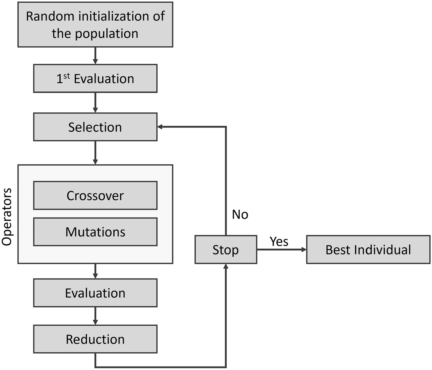
Genetic algorithm for searching in fragment spaces

Galileo is a classical GA operating on fragment spaces. A general workflow is shown in Fig. 1. The NAOMI framework [51] is used as the underlying cheminformatics engine.

Fig. 1

General workflow of Galileo. The fitness calculation is done either via an external fitness function or one of the integrated ones. Phariety has been directly integrated into Galileo

Representing fragment combinations

GAs require a representation for valid solutions to an optimization problem called chromosomes in this context. Traditionally, bitvectors have been applied for this task. There are several ways one could represent a molecule via a bitvector (e.g. by serializing the covalent bonds). In order to take a molecule’s fragmentation and corresponding connection rules into account, we represent molecules in chromosomes as fragment trees as described by Lauck et al. [7]: fragments (genes) are represented as vertices with potential attachment points that represent the linker atoms. Two vertices are adjacent if and only if the fragments are connected via a bond that is valid with respect to the connection rules. We consider any kind of molecule that may be created by such a combination of fragments a valid solution.

The optimization problem is defined by the scoring or fitness function assigning a numerical score (fitness) to each molecule in the solution set. They are described below.

Initialization

The population is randomly initialized. This is done by creating random fragment trees using the following procedure:

1.

pick a random fragment from the fragment space

2.

enumerate all linker atoms of this fragment

3.

retrieve all fragments from the fragment space that are compatible with at least one linker atom

4.

enumerate all fragment/compatible linker combinations

5.

select a random combination of fragment and linker atom

6.

attach the selected fragment to the corresponding linker atom

7.

repeat steps 2–6 considering all fragments in the tree until the tree is saturated (no open attachment points left) or until a user-defined number of fragments is reached

This randomized growing procedure is repeated until the desired population size is reached.

Crossover

Modern fragment spaces often contain a large number of connection rules. Many of these correspond to only a single reaction with a very specific chemical environment around the linker atoms. As such, the number of compatible linker types for any given linker type is orders of magnitude less than the number of linker types. A naive approach to perform a crossover between two chromosomes by randomly picking two chromosomes and randomly picking one edge each in both fragment trees is therefore unlikely to produce any valid offspring. We therefore decided on this alternative approach:

To perform a crossover between two chromosomes, all edges in the first Fragment Tree are enumerated. Each of these edges are considered in turn. The tree is cut along one of these edges. All edges of the second tree that have at least one attachment point that is compatible to either side of the cut are enumerated. For each of these compatible edges, the second tree is cut along that edge. Lastly, all combinations of subtrees of the first and second tree that result in valid Fragment Trees are created, resulting in anywhere between 1 and \(4 \cdot n \cdot m\) child trees, where n and m are the number of edges in the first and second Fragment Tree, respectively (see also Fig. 2). This is repeated for all pair-wise combinations of chromosomes in the selection (see below for the selection methods).

Fig. 2

Example of one possible crossover between Asp-Val and Cys-Phe dipeptides. The fragments are split along the peptide bond. Only two of the possible children are valid (Val-Phe and Cys-Asp). The other two children are invalid because the linker atom types are incompatible

To improve the performance of this step, we use an early-abort strategy where a chromosome combination is only considered if they have at least one compatible linker pair.

Mutation

Three mutation operators have been implemented, namely Replacement, Insertion and Deletion. All three modify a single fragment of a fragment tree, i.e. a single vertex or a gene in the GA context. They either replace an arbitrary fragment with a different compatible fragment, add a fragment to a linker atom or in between two other fragments, or remove a fragment with at most two adjacent fragments respectively. In case the removed fragment is connected to two fragments, these fragments must have compatible linker atoms such that they can be connected directly. An overview of the different possibilities is shown in Fig. 3.

Fig. 3

Mutation operations on a fragment tree. a Replacement of a fragment. Any fragment within a tree may be replaced; b i Addition of a terminal fragment; b ii Addition of a non-branching fragment; c i Deletion of a terminal fragment; c ii Deletion of a non-branching fragment. New fragments and edges are marked in solid green, removed ones are dashed in red

Replacement

Any fragment in a fragment tree may be replaced by another fragment that is compatible to all of the adjacent vertices of the original fragment. The procedure is as follows:

1.

Pick a random fragment from the fragment tree and remove it.

2.

For each new linker atom, select all fragments from the fragment space with at least one compatible linker atom.

3.

Calculate the intersection of all sets obtained in step 2.

4.

Filter out all fragments that have fewer linker atoms than the number of surrounding fragments.

5.

Remove the original fragment from the candidate set.

6.

Assign a probability to each candidate fragment that’s proportional to its similarity to the original fragment.

7.

Select a random fragment according to the probability mass function (PMF) from step 6.

8.

Consider the selected fragment: Calculate all valid linker atom assignments and pick a random one. If no valid assignment could be found, remove the fragment, adjust the PMF accordingly and go to step 7.

9.

Connect the new fragment according to the picked assignment.

Step 3 is required to remove all fragments that can never be a potential candidate because they can’t be connected to all surrounding fragments. Step 4 is required as there may be linker types that are compatible with more than one of the surrounding linker atoms. After having obtained all potential candidate fragments, the valid assignments have to be calculated, i.e a matching between the linker atoms of the candidate fragment and the linker atoms of the surrounding fragments. To calculate these matchings, we build an unweighted bipartite graph. The first set of vertices represents the linker atoms of the candidate fragment:

$$\begin V_ = \\} \end$$

(1)

The second set of vertices represents the linker atoms of the surrounding fragments:

$$\begin V_ = \\} \end$$

(2)

There is an edge (u, v) between two vertices if and only if the linker atom types of u and v are compatible with each other. An assignment for the fragment can then be obtained by calculating a maximum matching M on the described graph. The assignment is valid if and only if \(|M| = |V_1|\). If there is more than one valid assignment, all of them are considered.

The reasoning behind the similarity measurement in step 6 is to prevent the creation of extremely dissimilar compounds via mutation. For this we calculate the Tanimoto coefficient between the CSFP2.5 [26] fingerprints of the candidate fragments and the original fragment. We chose 2 and 5 as the lower and upper bounds because fragments are typically small in size and higher bounds would therefore result in very specific fingerprints. The fingerprints for the fragments are preprocessed and available in a database.

Insertion

The insertion operator enumerates all linker atoms and edges of a given fragment tree and picks one of them randomly. In case a linker atom was picked, the same growing procedure described above for the Initialization is performed to add a new terminal fragment. If an edge was picked, the tree is split at this edge and a random new fragment that is compatible to both linker atoms is chosen according to the procedure described in the replacement operator.

Deletion

A fragment may be deleted either if it is a terminal fragment or if it has exactly two adjacent vertices with compatible linker atoms. In the first case, the vertex is simply removed. In the second case, the fragment is removed and the surrounding fragments are connected via the now unused linker atoms.

Selection

A number of different classical selection methods were implemented, namely: Roulette Wheel Selection (RWS), Stochastic Universal Sampling (SUS), Rank Selection (RS), Tournament Selection (TS) and Random Selection (RAND). The first four have been exhaustively described in previous works [52]. RAND simply chooses a number of chromosomes from the population at random without considering their fitness. The chosen selection method selects a user-defined fraction of the current population which is copied over to the next generation. Afterwards, the offspring generated via the crossover procedure is appended to the new population (see Crossover). The rest of the population is filled with mutations of the Fragment Trees that are already present in the new population. To not completely lose the possibility of further exploration of the solution space, a user-defined fraction of the population is filled with new random fragment trees in the same way as during the initialization.

Scoring

Galileo provides an interface that allows arbitrary external programs to be used for scoring, as long as they fulfill four criteria: They

1.

are scriptable, i.e. they provide a command-line interface

2.

take an SDF file as input

3.

assign a positive score (incl. 0) to every molecule

4.

print the scores in the same order as the input molecules

Additionally, Galileo provides a number of built-in functions that may be used in addition to external programs. This includes the pharmacophore-mapping procedure described later, as well as a number of simple functions that model physicochemical properties. Each property is converted into a score employing one-dimensional Gaussians with a user-defined mean and variance. The supported physicochemical properties are:

molecular weight

calculated logP [53]

number of hydrogen-bond donors/acceptors

number of nitrogen/oxygen atoms

number of (aromatic) rings

The built-in functions also include the possibility to define a target molecule and score the population by Tanimoto similarity [54] to this target. As molecular fingerprints, ECFP4 [55] and CSFP2.5 [26] descriptors are available. All internal scoring functions may be combined and weighted. The combined score is calculated by a linear combination of the weighted scores, normalized by the sum of weights.

Pharmacophore mapping

In order to demonstrate the capabilities of Galileo with respect to 3D searching, we developed and implemented the pharmacophore mapping routine Phariety which is subsequently described. Just as Galileo, Phariety is built on top of the NAOMI framework [51]. The algorithm consists of three main steps, which are discussed in detail in the following paragraphs. In addition to the integration into Galileo, Phariety is available as an independent command line tool for pharmacophore search in virtual compound libraries.

Preprocessing

The first step of Phariety is a preprocessing step, during which unsuitable molecules are eliminated. In case only a molecule’s topology is given, a set of low-energy conformations can be generated using the tool Conformator [56]. Functional groups with specific interaction types are identified for every molecule. To ensure the compatibility with other pharmacophore mapping tools, like Catalyst, Phase and LigandScout [57,58,59], Greene’s algorithm [60] is used for the identification of hydrophobic interactions. For interaction types like hydrogen-bond donors and acceptors, aromatic interactions, and charged interactions, the NAOMI interaction model is used. The model was derived and extended from the interaction assessment used in FlexX [61]. The assessment is based on a geometric analysis of the overlap of interaction surfaces of two interaction partners and their deviation from optimal interaction geometries. The latter are defined by Rarey et al. [61]. The interaction surfaces of a functional group are used to describe the relative geometric position of possible interaction partners. A topology and geometry analysis of molecular substructures, as described by Bietz [62], is used to assign interaction points to functional groups. Direction vectors are also derived from the analysis of the geometric arrangement of the functional groups. After the assignment of corresponding interaction points to every functional group, a quick compatibility test is performed. Here, number and types of the generated interaction points of a given candidate are tested for their compatibility with the query pharmacophore feature points. The test verifies that the candidate structure contains at least the same number of interaction points of the same type for each interaction type of the query pharmacophore model. Note that the candidate structure may have more features than the query pharmacophore model, which offers the possibility of a partial mapping.

Mapping algorithm

The feature points of the query pharmacophore are mapped onto the interaction points of the candidate molecules using a depth-first walk with backtracking, a strategy introduced by Kurogi and Gunar [50]. This greedy algorithm starts with a randomly chosen query pharmacophore feature point and attempts to find a valid compatible interaction point of the candidate molecule. The algorithm places the query pharmacophore feature points in a random order and uses a classical backtracking strategy by assigning compatible interaction points of the candidate molecule one by one. The moment the algorithm runs out of options for a feature point it traces back one step and attempts to find an alternative mapping for the last feature point. The process stops when either a valid mapping is found for every point, or all possible combinations have been tested (see Fig. 4). It is possible to search for either the first or the best mapping. If the latter is chosen, the algorithm continues after the first valid mapping and enumerates all possible remaining combinations. The compatibility test between pharmacophore feature points and candidate molecule interaction points consists of a feature type check and a geometric check. The latter includes the comparison of all distances between the new matched feature point/ interaction point pair and the already mapped points. The deviation between the two distances in the pharmacophore query and the candidate molecule has to be less than or equal to the sum of the two radii of the involved query pharmacophore feature points plus an optional, user-defined tolerance value (see also Fig. A1).

Fig. 4

Workflow of Phariety’s mapping algorithm. Query pharmacophore model (top) with underlying ligand structure. X ia points stands for all interaction points of the corresponding type of a candidate molecule. The algorithm stops if one valid mapping is found or all possibilities are checked and no mapping can be found

Postfiltering

A subsequent post-filtering step is performed for all valid assignments. It consists of three tests which verify all constraints of the query pharmacophore model. First, the candidate molecule is transformed onto the query pharmacophore model using Kabsch’s algorithm [63, 64]. Afterwards, the first test checks whether the centers of the interaction points are localized within the spheres of the corresponding pharmacophore feature points, while allowing a user-defined deviation (see Mapping Algorithm above). The second test verifies whether potentially defined directions of query pharmacophore points are compatible with the corresponding, mapped interactions of the candidate molecule. The angle between the corresponding directions has to be less than a user-defined threshold. A special case are terminal and rotatable acceptor and donor interactions points. Those interaction points are rotated onto the query feature points before checking the angular constraint. Note that this may cause a minor deviation in the hydrogen coordinates of the returned conformation from the original. The third test verifies that the heavy atoms of the transformed candidate molecule do not overlap with exclusion volume spheres if any are defined in the query pharmacophore. The van-der-Waals radii of the heavy atoms are used for this overlap test. A partial overlap may be allowed by the user.

Score calculation

A score in the range of [0, 1] is calculated for mappings that pass all postfiltering steps, where 1 means an ideal mapping without deviation, and 0 means that no valid mapping is possible. The latter is only returned if one of the checks in the postfiltering step fails or no mapping can be found in the first place. The score is a weighted linear combination of two normalized terms: the distance deviation (\(s_\)) and the direction angle deviation (\(s_\)):

Let \(i \mapsto m(i)\) be the mapping of the query feature point i.

$$\begin s_ = \frac (r_i + r_j + \epsilon )} \cdot \sum _ |d_ - d_| \end$$

(3)

where \(r_i\) and \(r_j\) are the radii of query feature points i and j, \(d_\) is the distance between the query feature points i, j and \(d_\) is the distance between the mapped interaction points m(i), m(j) of the candidate molecule.

$$\begin s_ = \frac \cdot \sum _ \angle (v_i, v_) \end$$

(4)

where n is the total number of regarded angles between direction vectors, \(\angle (v_i, v_)\) is the smaller angle between the direction vector \(v_i\) of the query feature point i and the direction vector \(v_\) of its mapped interaction point m(i) of the target.

The weights are user-defined and must add up to 1.0. The weight of the angle deviation term is set to 0.0 if no direction information exists. Per default, both weights are set to 0.5. The final score is given by:

$$\begin s_ = 1 - (w_ \cdot s_ + w_ \cdot s_) \end$$

(5)

where \(w_\) is the weight for the distance deviation term and \(w_\) is the weight for the angle deviation term.

The algorithm returns a score for each candidate molecule and, if possible, the corresponding conformation superposed onto the query pharmacophore model.