In the operation of machinery, bearings are often one of the most easily damaged parts due to the high frequency of use. And because the bearing generally plays the role of supporting the main shaft and transmitting the torque, it plays a decisive role in whether the equipment can work normally. Once the equipment fails, it may lead to catastrophic consequences, so it is particularly important for bearing fault diagnosis (Liu, 2017; Du et al., 2020; Li et al., 2020; Yu et al., 2020). When the bearing fails, the vibration signal generated has certain characteristics. The fault diagnosis of the bearing is to classify the collected vibration signal. The traditional diagnosis process is to extract relevant features from the collected vibration signals, and then use a specific classifier to classify and identify. For example, In 2020, researchers such as Yang et al. (2020) used wavelet packets to extract bearing fault features and input the obtained feature information into an improved Bayesian classification model for classification. The experimental results show that compared with the model before optimization, the modeling time is shorter and the fault diagnosis accuracy is higher. In 2020, researchers such as Wang et al. (2020) proposed a rolling bearing fault diagnosis method based on minimum entropy deconvolution (MED) and Autogram. This method removes noise through MED, and can effectively highlight fault features while obtaining the best frequency band. Compared with the existing methods at that time, it can detect the demodulation frequency band and fault frequency more accurately, highlight the fault characteristics and improve the fault detection effect. In 2021, researchers such as Zhen et al. (2021) proposed a bearing fault signal feature extraction method based on the combination of wavelet packet energy and kurtosis spectrum. This method can clearly obtain the fault characteristic frequency and its higher harmonics.

It can be seen from the existing research results that this kind of bearing fault diagnosis method can effectively extract features and classify them. However, it is necessary to manually extract features, which requires a large workload and subjective factors. Therefore, it is limited in practical application. In order to solve these problems, the study of deep learning in bearing fault diagnosis has attracted extensive attention of researchers. Deep learning is an end-to-end recognition method, which can extract features adaptively, and better solve the defects of manual feature extraction. In 2018, researchers such as Qu et al. (2018) proposed a fault diagnosis algorithm based on an adaptive one-dimensional convolutional neural network. Features are extracted through the convolution and pooling layers of the convolutional neural network, and classified through the Softmax layer. In 2020, researchers such as Gu et al. (2020) proposed an adaptive one-dimensional convolutional neural network and long short-term memory network fusion bearing fault diagnosis method. This method improves the accuracy as well as the validity and stability of the model. In 2021, researchers such as Liu et al. (2021) proposed a fault diagnosis method for rolling bearings based on parallel 1DCNN. Improve the ability of fault diagnosis by fusing time domain and frequency domain features, This method can make full use of the extracted time domain and frequency domain feature information, and has better fault diagnosis ability.

Judging from the existing research progress, the research on bearing fault diagnosis based on deep learning has achieved good results, which can achieve accurate identification of bearing fault diagnosis. However, the generalization and robustness of the existing diagnostic models still need to be improved. In view of these research problems, this paper designs a convolutional neural network model based on particle swarm optimization fusion. Optimizing the network’s hyperparameter learning rate through PSO (Particle Swarm Optimization) enables the network to achieve a better gradient global minimum in the gradient descent process, And introduce residual connections to alleviate gradient disappearance, Then use global average pooling to replace part of the fully connected layer to reduce the amount of parameters and improve generalization, Finally, a Dropout layer is added to prevent the network from overfitting.

Convolutional neural networks have the characteristics of end-to-end, local perception and parameter sharing. Feature extraction is performed on the input data through multiple filters. When the network is deepened, the extracted features are also more advanced, and robust features with shift invariance are obtained in the original data. Compared with models that extract features manually, convolutional neural networks have stronger discriminative and generalization capabilities. It can effectively obtain the local features of the data to be tested, and is widely used in classification problems such as image processing, speech recognition, and natural language processing (Maite et al., 2020; Tian, 2020; Wang et al., 2021; Chen et al., 2022; Sultana et al., 2022).

Convolutional neural networks are composed of convolutional layers, pooling layers, fully connected layers and output layers. The convolutional layer and the pooling layer perform feature extraction on the input data. The mathematical model of the convolution operation of the convolution layer can be expressed as:

yij=f⁢(∑i=1∑j=1xij⁢wij+b)(1)

Among them, yij is the output, xij is the input, wij is the weight value, b is the bias, and f() is the activation function. The purpose of the activation function is to make the input not a linear function so that it can approximate any function and make the network generalization ability stronger. The activation function generally adopts the Relu function and its mathematical expression is:

f⁢(x)=max⁢(0,Y)(2)

Among them, f(x) is the output, and Y is the activation value that the convolutional addition will add the bias value.

The pooling layer is mainly divided into maximum pooling and minimum pooling, and its mathematical models can be described as:

ymax=max⁢(x11,…⁢xij)(3)

ymean=mean⁢(x11,…⁢xij)(4)

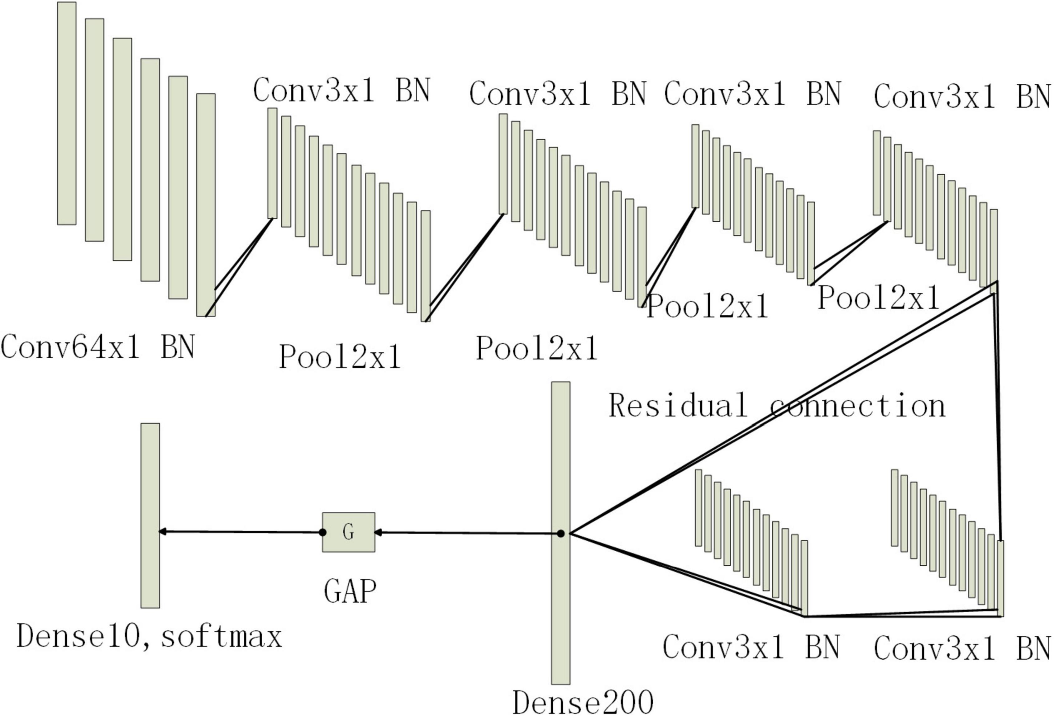
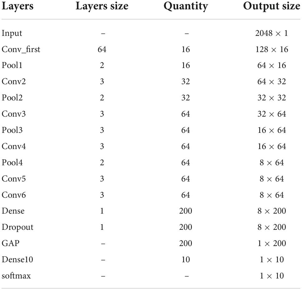
Among them, ymax and ymean is the pooling output.xij is the output value at position (i, j) that take the maximum value or average value in the pooling area for output. After multiple convolution and pooling layers, the input fully connected layer fuses the learned features and maps them to the label space. Finally, the classification results are output through the Softmax function in the output layer. Since the bearing fault data is one-dimensional amplitude data, this paper will use the backbone of the convolutional neural network as a one-dimensional convolutional neural network. The convolution kernel is a one-dimensional structure, and the output of each convolutional layer and pooling layer will be a one-dimensional feature vector. The first layer of the convolutional layer uses large convolution kernels and large steps to increase the field of view of this layer, which can effectively extract the overall timing features. Then, a small convolution kernel is used to deepen the network. In order to avoid the risk of gradient disappearance as the network deepens, this paper will introduce a residual structure. Then replace some of the fully connected layers with global average pooling. Compared with the fully connected layer, the global draw pooling can greatly reduce the training parameters and speed up the training speed, while enhancing the generalization of the network and preventing overfitting. A BN operation is added to each convolutional layer. It can play the function of controlling the gradient explosion or gradient disappearance. Finally, a Dropout layer is added to prevent the network from overfitting. Its network structure is shown in Figure 1, Table 1. Conv represents the convolution layer, Pool represents the pooled layer, Dense represents the fully connected layer, BN represents the batch normalization layer, and GAP represents the global average pooled layer. The following numbers represent the convolution core size and x1 represents the one-dimension.

Figure 1. Network structure diagram.

Table 1. Model structure parameters.

In order to improve the performance, when training the convolutional neural network, it is necessary to set certain hyperparameters for the network. If the hyperparameters are manually set, it will take a long time and lack generalization to different scenarios. Due to its advantages of easy convergence and strong global search ability, particle swarm optimization method is very suitable for hyperparameter optimization of machine learning algorithms (Shao et al., 2020; Li et al., 2022). The training of the convolutional neural network model is the process of finding the lowest point of the gradient. In order to better obtain the lowest point of the global gradient, the setting of the learning rate is particularly important. When the learning rate is set too large, it will miss the global optimal solution or fail to converge at all, and a better training structure cannot be obtained. When the learning rate is set too small, the convergence of the model will be very slow, and the model may be unable to jump out of the local optimal solution. The artificial setting of the learning rate will be objective, and it is impossible to give a good value in different model use cases. Therefore, this paper introduces the PSO particle swarm algorithm to set an adaptive setting for the hyperparameter learning rate.

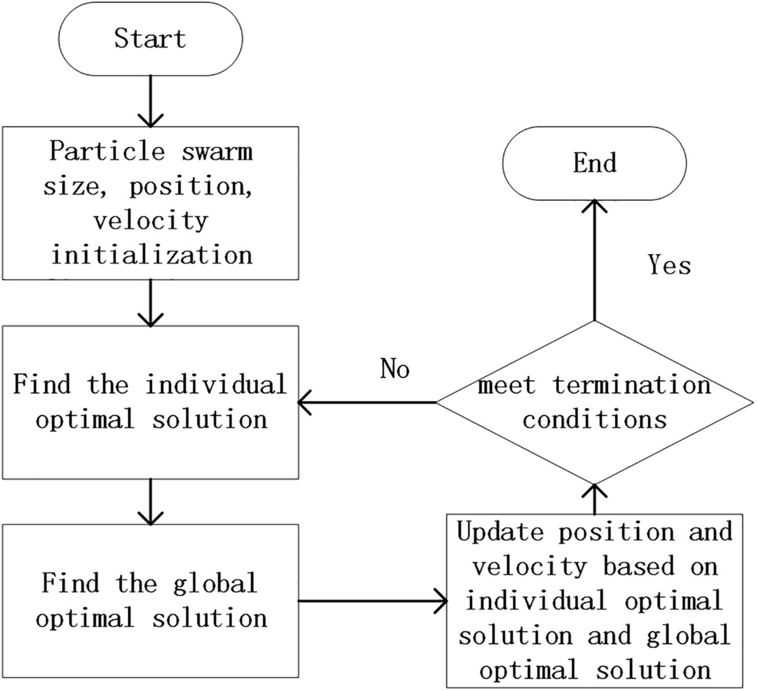
Particle swarm optimization is to generate a group of particles in the space that needs to be solved, and each particle has two attributes of velocity and position. Among them, the speed represents the speed of the movement, and the position represents the direction of the movement. Each particle searches for the optimal solution individually in space, and records it as the current individual best solution to obtain the local optimal solution Pbest, and then shares all individual extreme values with other particles in the entire particle swarm. A global optimal solution Gbest is selected from the individual optimal solutions of the particle swarm, and all particles adjust their speed and position according to the individual optimal solution Pbest and the global optimal solution Gbest. Its process is shown in Figure 2.

Figure 2. Particle swarm optimization flowchart.

The update formula of particle position and velocity of particle swarm is:

,,,]},,,]},,,]},,,,,]}],"socialLinks":[,"type":"Link","color":"Grey","icon":"Facebook","size":"Medium","hiddenText":true},,"type":"Link","color":"Grey","icon":"Twitter","size":"Medium","hiddenText":true},,"type":"Link","color":"Grey","icon":"LinkedIn","size":"Medium","hiddenText":true},,"type":"Link","color":"Grey","icon":"Instagram","size":"Medium","hiddenText":true}],"copyright":"Frontiers Media S.A. All rights reserved","termsAndConditionsUrl":"https://www.frontiersin.org/legal/terms-and-conditions","privacyPolicyUrl":"https://www.frontiersin.org/legal/privacy-policy"}'>