
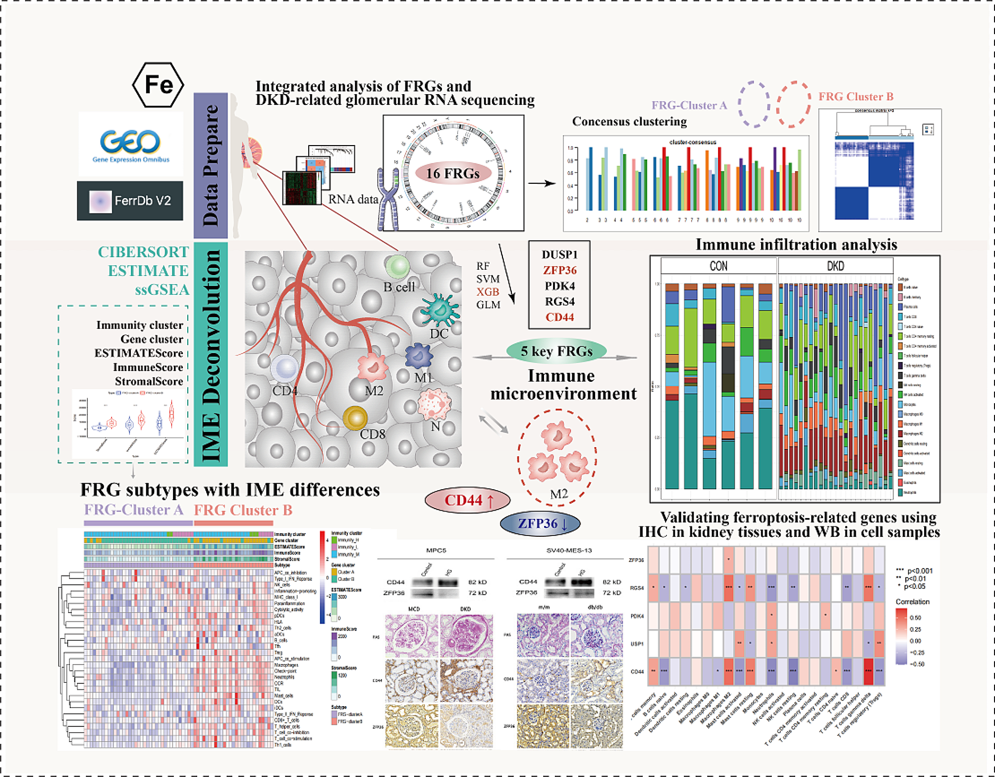
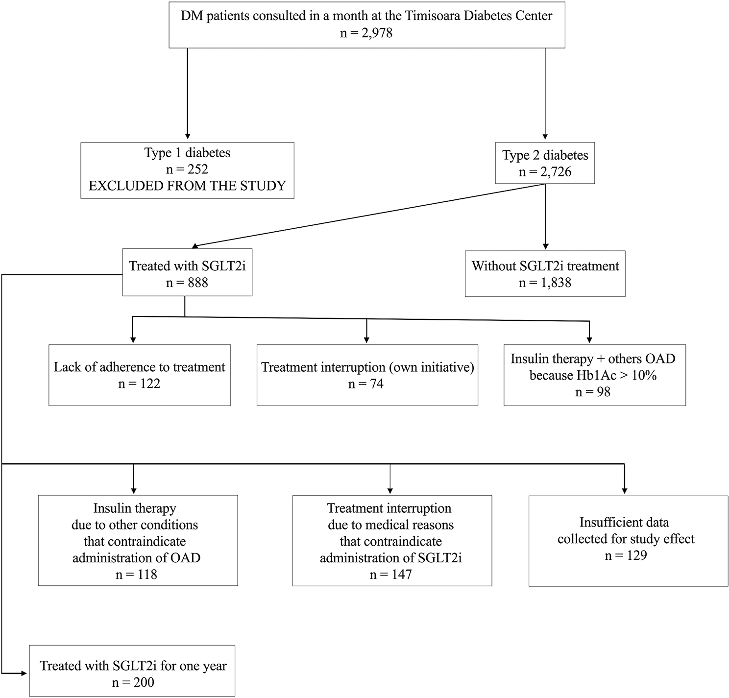
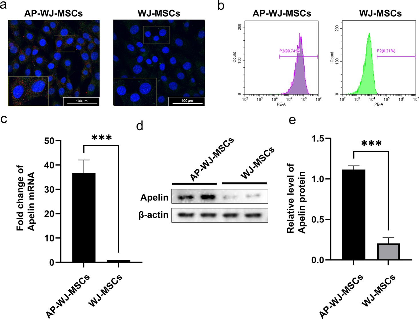
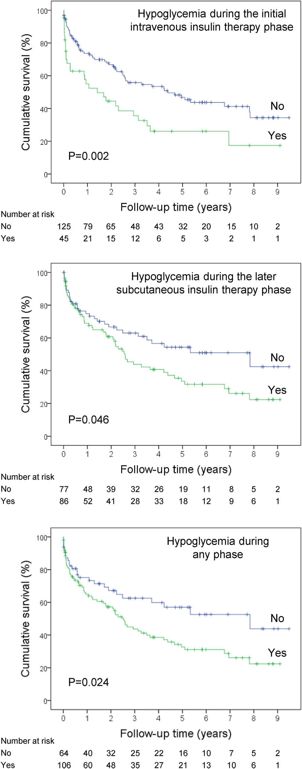
記住我
Images were taken from wild-type control mice in 2 different diet studies on genetically modified male mice [15, 16]. The mice were fed either a control (low-fat, LF, 3.8 kcal/g) or high-fat (HF, 4.7 kcal/g) diet for 10 weeks. Further details are presented in Additional file 3. MRI was performed in the kidney area with a 7 T small animal magnetic resonance tomograph with ParaVision 5.1 software (Bruker Biospin MRI Gmbh, Billerica, Massachusetts, USA). A series of axial base images (“base image”) were acquired with T1-weighted Rapid Acquisition with Relaxation Enhancement (RARE), and fat suppressed images (“water image”) were acquired in the same spatial domain with Chemical Shift-selective Fat Suppression (CHESS). Water suppressed images (“fat image”) were acquired by subtracting the water images from the base images. The image size was 256 × 256 voxels, with each voxel measuring 0.156 × 0.156 × 1 mm. Both MRI and glucose tolerance tests were performed in the last 3 weeks of the diet period. For the CD1 mice, glucose tolerance tests were performed by feeding the mice 2 mg/g glucose orally via tube. Blood glucose was measured at 0, 15, 30, 60, 120 and 240 min. The C57BL/6 J mice had glucose injected intraperitoneally, and blood glucose was measured at 0, 15, 30, 60, 120 and 180 min.
Human images were acquired from healthy subjects by a 2-point Dixon sequence performed on a 1.5 T Siemens Avanto running Syngo MR B17 (Syngo, Siemens, Erlangen, Germany), giving two groups of images in the same spatial domain; with the water and fat spins in-phase or out-of-phase, which is used to generate water and fat images [17]. The image size was 320 × 240 voxels, with each voxel measuring 1.234 × 1.234 × 2.5 mm.
For each mouse and each human subject, respectively, 10 sequential images in the kidney area were selected for segmentation. The kidney is located in approximately the same area in all subjects within each species, and is therefore well suited as an anchor point when comparing adipose tissue volumes. An approximate midpoint of the kidneys was found where there was an equal number of images on each side with at least 1 kidney visible. The 10 sequential images selected for volume quantification were the 5 closest images on each side of this midpoint.
R packagesThis protocol was developed with R 3.6.3 in RStudio 1.2.5033 (RStudio, PBC, Boston, Massachusetts, USA). Functions are shown in cursive, and the package given in parentheses when not a basic R function. The package oro.dicom [18] was used for loading dicom files into R. Most of the functions used here are from EBImage [19] and imager [20]. The tidyverse [21] collection of packages were used for data handling and output formatting. A short description of fat segmentation is presented in Fig. 1. For a detailed protocol and further information about the packages, see Additional files 1, 2.
Fig. 1
Overview of the workflow of fat segmentation of MRI images with RAdipoSeg. The procedure begin by finding and removing background noise, and thresholding the image. Removal of some voxels may be necessary to divide SAT from VAT, if the depots lie so close together that there is no line of black voxels between them in the image. Finally the objects are selected to the different depots and volume is calculated
Background noise and thresholdingThe margins of each image were divided into 8 fields and the background noise calculated from randomly selected voxels from these fields. If some fields had high signal objects, e.g., arms, they were removed and the voxels were randomly selected from the remaining fields. The background noise (BG) was calculated as the sum of the mean and standard deviation (sd) of the voxel intensities. If objects with high signal intensity were not removed, the background noise was too high for use in further calculations.
Thresholding was used to separate objects representing adipose tissue from the rest of the image. Thresholding works by setting all voxels above or equal to a set signal intensity (the threshold) to 1 and all voxels below the threshold to 0. The threshold value was calculated from the voxel intensities along the contour of the body. The contour is the line of voxels which separates the body from the background in an MRI image. In an axial water suppressed image (fat image), a large portion of the voxels along the contour represent SAT. To find the contour, we used the base images for the mice and the in-phase images for the humans, which were thresholded using a modified version of Otsu’s method [22]. Then a contour finding algorithm was applied using ocontour (EBImage). The adipose tissue threshold for the fat images was found by subtracting sd from the mean of the intensities. When this value was below the calculated background noise, the threshold was recalculated as TC = BG + 0.1 × sd, where TC is the threshold, BG is the background noise and sd is the standard deviation of the voxel intensities, as described previously [10]. The fat images were then thresholded using thresh (EBImage). This function performs local thresholding using a moving rectangular window and TC as the offset value. The size of the rectangular window was optimized as 15 × 15 voxels for mouse images and 50 × 50 for human images.
The background noise was removed with a mask created using fillHull and floodFill (EBImage), which set all voxels outside of the mask to 0.
Labelling image objects, manual editing, and volume estimationSome images were edited manually for removal of areas (e.g., bone marrow) and then the images were labelled using bwlabel (EBImage). This function gives each piece of interconnected voxels a separate value, counting the objects. To distinguish SAT from VAT, it was necessary to divide some objects by manually setting voxels to 0, and then relabel the image. These voxels were automatically reinserted to the appropriate depot later to avoid loss of data. Voxels can also be manually added or deleted to correct for incomplete fat suppression caused by inhomogeneties in the magnetic field during scanning. However, this was not performed on these images. The selection of objects was achieved by using grapPoint (imager). New images were made with all SAT having voxel value 1 and VAT value 2, and the volumes were calculated by counting the voxels.
Method evaluationTo evaluate the method, fat segmentation was performed on the same images with SliceOmatic’s region growing mode. Selections of the segmented images from both methods were validated by a radiologist. The volumetric overlap errors were calculated with the Jaccard distance [23], given as 100(1− (|A ∩ B|/|A ∪ B|), where 0% is a perfect overlap between segmentation by RAdipoSeg and SliceOmatic. The relative volume differences (RVD) between RAdipoSeg (A) and SliceOmatic reference (B) were calculated as 100((|A|− |B|)/|B|). Spearman’s rank correlation coefficients were calculated to test for linear correlation. Bland–Altman analyses were performed with differences between the methods on the y-axis and mean of the methods on the x-axis, and with 95% confidence intervals. Proportional bias was tested using Spearman’s rank correlation coefficients on the data from the Bland–Altman analyses. Normalcy was assessed by Shapiro–Wilk test. All statistical analyses and making of plots were conducted in R. The figures were created in Inkscape 1.0.0 (https://inkscape.org/), with text size being the only alteration made to the plots.
留言 (0)