Introduction

Functional near-infrared spectroscopy (fNIRS) is a non-invasive brain imaging technique that uses near-infrared light (typically of wavelengths between 650 and 1,000 nm) to monitor hemodynamics changes in the cortical layer. Compared to electroencephalography (EEG), fNIRS enables to measure brain-activity related hemodynamics in terms of cerebral oxygenation and is less susceptible to electric noises (Huppert et al., 2009; Tak and Ye, 2014; Naseer and Hong, 2015; Chiarelli et al., 2017; Afkhami et al., 2019; Ghafoor et al., 2019; Khan et al., 2021). In addition, fNIRS can be integrated into a portable, wearable, and ergonomic device at low costs and operational expenses, making it a superior candidate for a user-friendly brain-computer interface system compared to other modalities, such as functional magnetic resonance imaging (fMRI) and magnetoencephalography (MEG) (Hu et al., 2010; Piper et al., 2014; Scholkmann et al., 2014a; Pinti et al., 2015; Wyser et al., 2017; Zhao and Cooper, 2018; Hong and Zafar, 2018; Zhao H. B. et al., 2020, 2021; Ghafoor et al., 2021; Huang and Hong, 2021).

Fantini et al. (1999) reported that the artifacts caused by subjects’ movements, specifically motion artifacts (MAs), can significantly influence the quality of the recorded optical signals of fNIRS. Some studies claimed that MAs reduce the signal-to-noise ratio (SNR) of fNIRS signals (Izzetoglu et al., 2005; Izzetoglu et al., 2010). Researchers have also verified that using MA removal techniques can ameliorate classification accuracy in cognition experiments (Zhou et al., 2021). Therefore, the issue concerning the causes, characteristics, and rejection methods of MAs in fNIRS signals is a crucial topic in fNIRS studies (Safaie et al., 2013; Piper et al., 2014).

During the early days, researchers skipped the analysis or discarded the data set when the measured signals were significantly corrupted by motion artifacts (Bartocci et al., 2000; Jasdzewski et al., 2003; Akgul et al., 2005; Khan and Hong, 2015; Nguyen and Hong, 2016; Zafar and Hong, 2017). Schroeter et al. (2003) removed the outliers manually. Moosmann et al. (2003) eliminated the disturbances by immobilizing the subjects’ heads with a vacuum pad. Subsequently, a moving average was used (Kameyama et al., 2004; Lee et al., 2007). Channel rejection is another common method in early studies (Wilcox et al., 2005; Blasi et al., 2010). Attempts were made to remove MAs using an improved optical model. Nevertheless, the performances of the aforementioned solutions were not sufficient (Scholkmann et al., 2014b). Nowadays, a correction for motion artifacts has become a common consensus: Some processed the signals in two stages: artifact identifications and artifact corrections in the existing methods (Scholkmann et al., 2010; Virtanen et al., 2011; Yucel et al., 2014a), or minimized a user-defined cost function (Kim et al., 2011), or proposed a new model to compensate the artifacts (Izzetoglu et al., 2010; Yamada et al., 2015).

The existing literature indicates that the movements that cause MAs are diverse. Several studies have reported that the movements of subjects’ heads (including nodding, shaking, tilting, etc.) could result in MAs in fNIRS measurements (Izzetoglu et al., 2005; Radhakrishnan et al., 2009; Robertson et al., 2010; Kim et al., 2011; Cui et al., 2015). Some researchers further discovered that facial muscle movement, including raising eyebrows, can lead to MAs (Izzetoglu et al., 2005; Robertson et al., 2010; Yucel et al., 2014b; Zhou et al., 2021). In addition, body movements, including the movement of the upper and lower limbs, degrade the fNIRS signals by causing head movements or by the inertia of the device (Yucel et al., 2014a; Rea et al., 2014; Abtahi et al., 2017; Vitorio et al., 2017; Khan et al., 2018; Siddiquee et al., 2020; Dybvik and Steinert, 2021). Vinette et al. (2015) monitored five epilepsy patients for a long period. Their data showed that MAs existed when the subjects were talking, eating, or drinking. These behaviors involve jaw movements. Novi et al. (2020) found that jaw movements could lead to two different motion artifacts. The direct cause of MAs is imperfect contact between the optodes and the scalp, including displacement, non-orthogonal contact, and oscillation of the optodes (Yamada et al., 2015; Nishiyori, 2016).

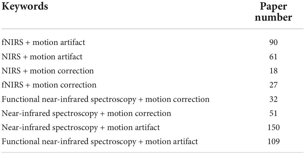
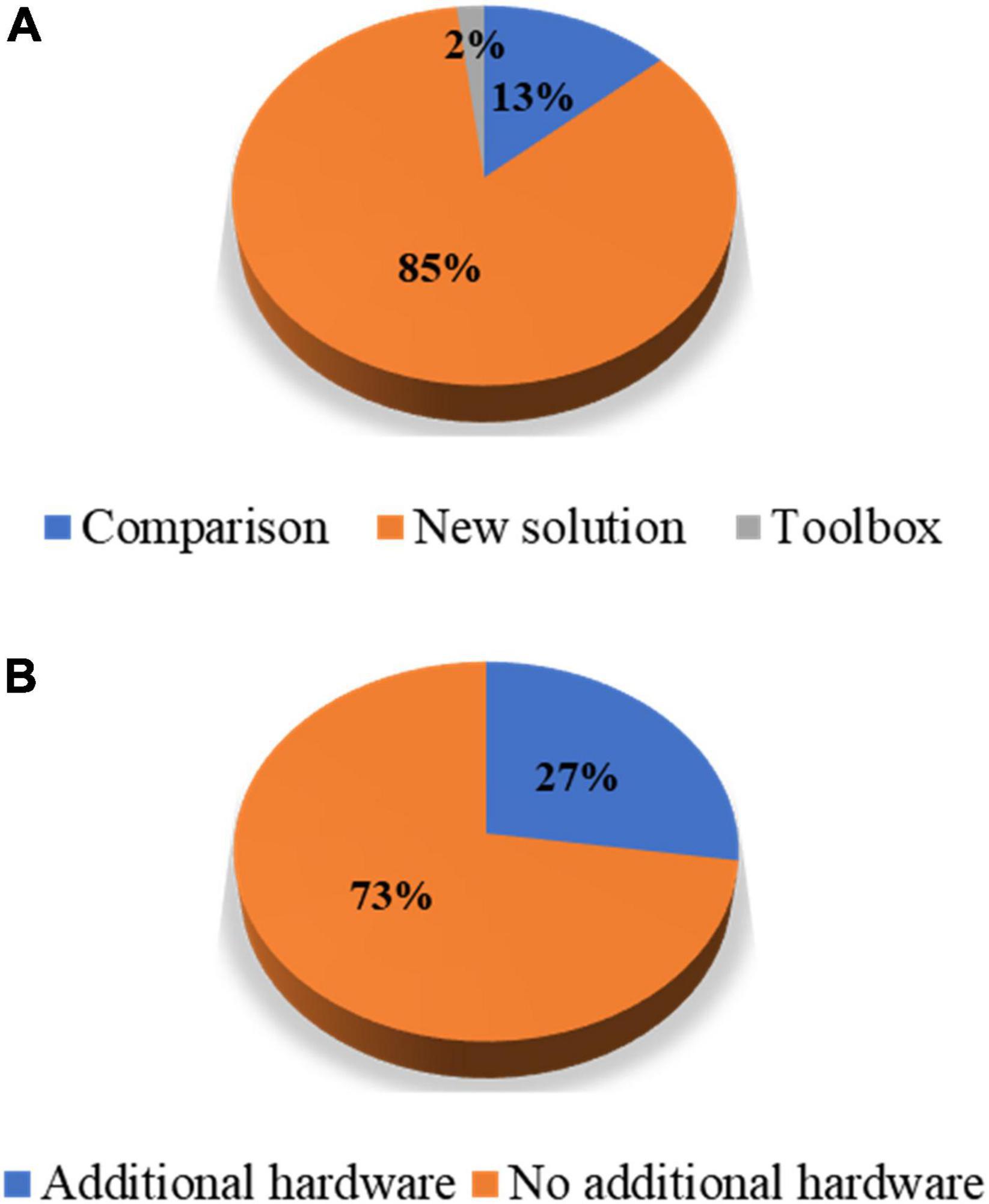
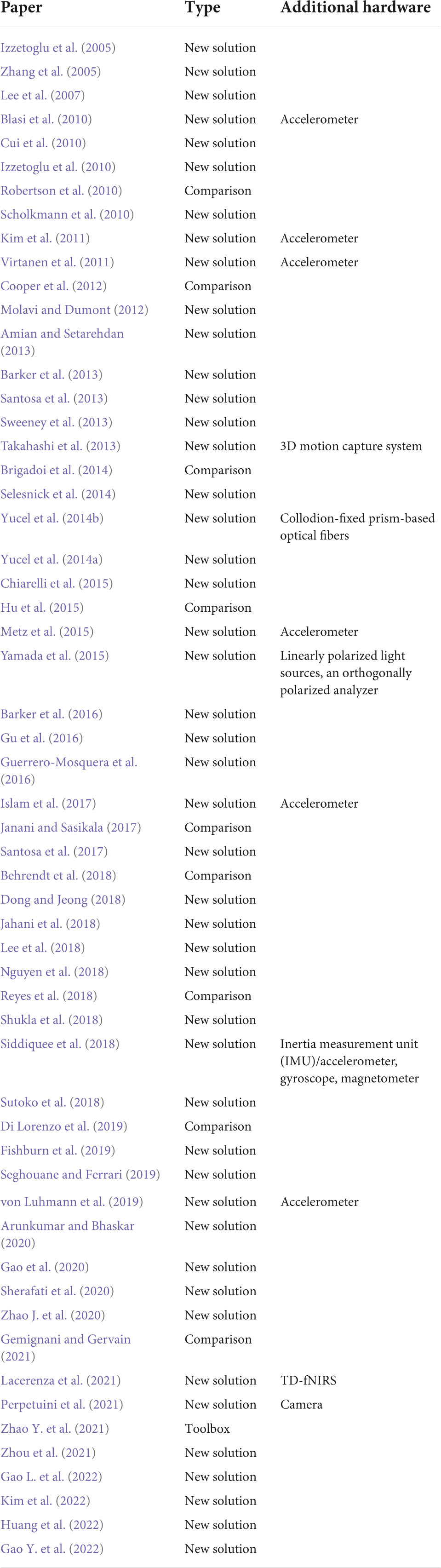
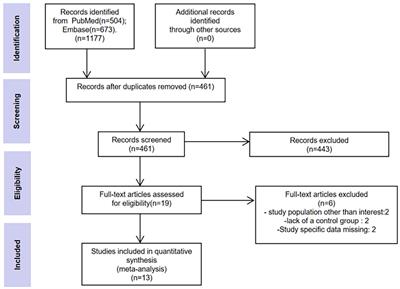
In this study, the authors reviewed journal articles concerning MA removal techniques in the Web of Science database. The keywords and numbers of journal papers are listed in Table 1. To narrow down our review scope, we list all journal articles found in the database. Subsequently, all the overlapping papers and irrelevant articles were removed by examining their context, which yielded 89 papers. Next, we proceeded to select journal papers that satisfied at least one of the following criteria: (i) The paper proposes a novel MA removal technique; (ii) the paper presents a quantitative comparison of several MA removal techniques; and (iii) the paper introduces a toolbox for MA removal. Eventually, 55 papers were selected from the literature. Forty-three papers presented a new solution to suppress MAs, seven papers compared the performance of the existing methods, and one study introduced a toolbox. Figure 1 shows the partitioning of different types of papers in the selection process. Among the 47 new solutions, twelve solutions added auxiliary hardware. A list of selected studies and their categories is presented in Table 2. Since research on MA removal techniques requires a solid foundation in mathematics and programming, it is difficult for new scholars to assimilate the existing solutions in their studies. Moreover, some solutions were described in the text rather than using equations, making it difficult for other researchers to reproduce the reported methodologies. Therefore, this study aims to (i) provide a general view of the latest achievements in MA removal studies, (ii) briefly introduce several significant solutions from the view point of application and reproduction by using equations, and (iii) discuss future topics in the field.

TABLE 1

Table 1. The number of journal papers (1990∼2022) obtained from the Web of Science database by combining different keywords.

FIGURE 1

Figure 1. Percentage partitions: (A) Article types of the selected papers and (B) hardware-based solutions against algorithmic solutions among the papers proposing new solutions.

TABLE 2

Table 2. List of selected papers, article types, and information on additional hardware.

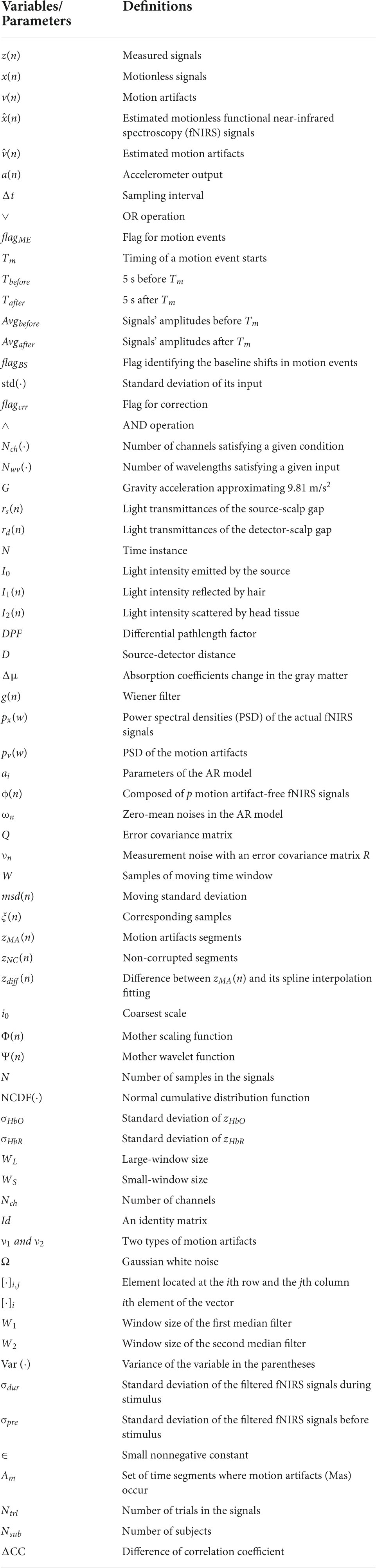
This study is divided into five sections. The “Introduction” section presents the causes and significance of MA issues in fNIRS. In addition, this section specifies the objectives of this study and provides a quantitative summary of the existing literature on the topics. The section “Additional hardware-based techniques” summarizes the existing hardware-based solutions. The section “Signal processing-based techniques” discusses the algorithmic solutions. The section “Evaluation metrics” briefly introduces the definitions of some metrics to evaluate the performance of MA removal techniques. The final section “Conclusions and outlook” concludes this study and discusses potential issues concerning MA removal. We will use the compact notation provided in Table 3 for the remainder of the paper.

TABLE 3

Table 3. Definitions of variables, parameters, and their values.

Additional hardware-based techniques

Among the eight-nine selected papers, 17 discussed solutions using additional hardware, while 11 studies discussed accelerometer-related methods. Other auxiliary hardware includes a headpost cemented to the skull, a three-dimensional (3D) motion capture system, collodion-fixed prism-based optical fibers, an inertia measurement unit (IMU), a gyroscope, a magnetometer, and a camera. This section presents two solutions using accelerometers and one using linearly polarized light.

Accelerometer

Accelerometer-based methods include adaptive filtering, active noise cancelation (ANC) (Kim et al., 2011), accelerometer-based motion artifact removal (ABAMAR) (Virtanen et al., 2011), acceleration-based movement artifact reduction algorithm (ABMARA) (Metz et al., 2015), multi-stage cascaded adaptive filtering (Islam et al., 2017), blind source separation, accelerometer-based artifact rejection, and detection (BLISSA2RD) (von Luhmann et al., 2019). The introduction of the accelerometer improves the feasibility of real-time rejection of MAs.

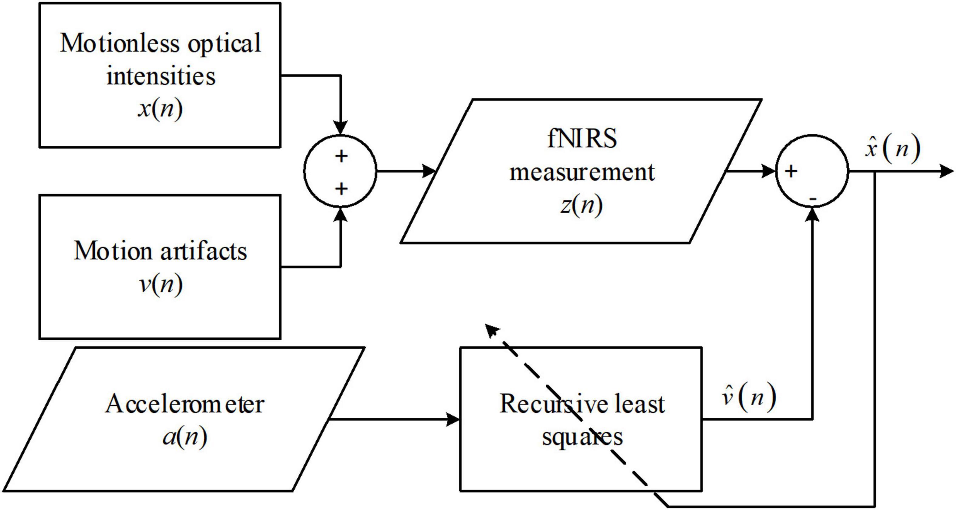
Active noise cancelation

The method assumes that the measured signals, z(n), are the sum of motionless signals, x(n), and MAs, v(n) (Kim et al., 2011). The objective of the solution is to minimize the power of the recovered signals, that is,

min⁡(E(x^(n)2))=min⁡(E((x(n)+v(n)-v^(n))2))

                            =min(E(x(n)2)+2E(x(n)v(n))

                                                                             -2E(x(n)v^(n))+E((v(n)-v^(n))2)).(1)

where E(⋅) denotes the expectation function, and the hat over x and v denotes the estimation of motionless fNIRS signals and MAs. Ideally, x is uncorrelated to either v or the estimate of v. Therefore, the two cross-terms on the right-hand side are equal to zero implying that the objective is equivalent to minimizing the square difference between the MAs and the estimated MAs. Moreover, because the actual MAs are highly correlated to the accelerometer output, a(n), but unknown to users, v(n) is replaced by a(n) in the application. Subsequently, the final objective of signal processing is to minimize the square difference between a(n) and the estimated MAs, that is,

min⁡(E((a(n)-v^(n))2))(2)

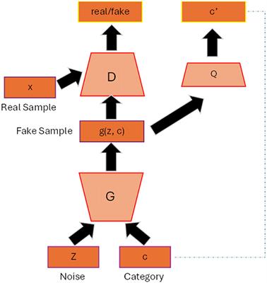
The estimate of v(n) can be obtained using the difference between z(n) and the estimate of x(n). The estimate of v(n) can then be computed in real time using a recursive least-squares filter. The procedure for the solution is graphically presented in Figure 2. The ANC solution was applied to optical intensities in real time. Whether this method was applied to optical densities or concentration changes is not clear. Another issue in the approach of Kim et al. (2011) is that the performance was visually evaluated. Therefore, a quantitative evaluation of ANC in the sense of both noise suppression and signal distortion is needed.

FIGURE 2

Figure 2. Procedures of active noise cancellation (ANC) algorithm.

Accelerometer-based motion artifact removal algorithm

The ABAMAR method is an offline analysis method for MA removal, where accelerometer outputs are used for MA detection, and the MA removal process is based on the measured fNIRS signals (Virtanen et al., 2011). Accordingly, we first define two Boolean functions as follows.

f1(x)={1x≥00x<0(3)

f2(x)={1x>00x≤0(4)

A motion event can then be identified using the acceleration at the x- and y-axes, where Δt is the sampling period. The subscript x or y at a(n) denotes the acceleration at the two axes. The subscript ME denotes the motion event, and operator ∨ denotes the OR operation. The flag for the motion events can be computed as follows.

flagME=f1(|ax(n)-ax(n-1)|-1.3ΔT)∨f1(|ay(n)-ay(n-1)|-1.3ΔT)(5)

If flagME is one, the signals encounter a motion event; otherwise, zero. Once a first true value of the flag appears, the timing of the motion event starts and is stored/defined as Tm. The motion event is ended when the flag remains false for over 20 s. The ending time is identified as the last sample when flagME is true.

Another flag, flagMA, is introduced to identify the existence of MAs, which is defined as follows.

flagMA=f1(Tm-1)(6)

Tm is the starting time of a motion event. The baseline of fNIRS signals, Avg, is defined as the average of the signal amplitudes before and after Tm. To avoid disturbance during the motion event, we marked 5 s before Tm as Tbefore and 5 s after Tm as Tafter. The amplitudes of the signals before Tm, Avgbefore, and those after Tm, Avgafter, are calculated as follows.

Avgbefore=mean(z(n)|Tbefore-15≤n<Tbefore)(7)

Avgafter=mean(z(n)|Tafter<n≤Tafter+15)(8)

flagBS is a flag identifying baseline shifts in motion events. Specifically, one for baseline shifts, and zero for no shift.

flagBS=f2(|Avgbefore-Avgafter|-2.6σbefore)(9)

σbefore=std(z(n)|Tbefore-15≤n<Tbefore)(10)

The function std(⋅) computes the standard deviation of its input.

The correction procedure only applies to baseline shift segments. Moreover, a flag for correction, flagcrr, is introduced. If its value is one, a correction of signals will be conducted; otherwise, it is zero. Moreover, operator ∧ denotes the AND operation. The flagcrr can be computed as follows.

flagcrr=f1(Nch(flagBS|flagBS=1)-2)∨f1(Nwv(flagBS|flagBS=1-2))∧flagME(11)

where Nch(⋅) denotes the number of channels satisfying the condition specified in the input, and Nwv(⋅) denotes the number of wavelengths satisfying the input. When flagcrr is one, z(n) is corrected as follows.

z^(n)|nafterTm=AvgbeforeAvgafterz(n)(12)

z^(n)|ninsideTm=Abefore(13)

The ABAMAR solution is applied to optical intensities, optical densities, and concentration changes. It can efficiently suppress step-like artifacts. However, the signal details during motion events will be lost owing to the correction method. Moreover, empirical constants, such as 1.3 g/s in Eq. (5) (g denotes the gravitational acceleration of 9.81 m/s2) and 2.6 in Eq. (9), may need to be updated for tasks other than sleeping monitoring. Some researchers have proposed an AMARA, which is an improvement of ABAMAR (Metz et al., 2015), by combining the movement artifact reduction algorithm (MARA; see section “Spline interpolation”) and ABAMAR.

Linearly polarized light-based solution Multidistance optode arrangement technique

An optical model of light transmission between a source and a detector is developed using light transmittance (Yamada et al., 2015). Here, the light transmittances of the source-scalp gap, detector-scalp gap, and head tissue at time instance n are denoted by rs(n), rd(n), and R(n), respectively. Moreover, the light intensity emitted by the source is denoted by I0, the light intensity reflected by the hair is denoted by I1(n), and the light intensity scattered by the head tissue is denoted by I2(n). The optical density can then be computed as follows.

ΔA (n)=-I1(n)+I2(n)I1(0)+I2(0)

                                           =-log⁡I1(n)+I0rs(n)R(0)rd(n)I1(0)+I0rs(0)R(0)rd(0)

                                                                              -log⁡I1(n)+I0rs(n)R(n)rd(n)I1(n)+I0rs(n)R(0)rd(n),(14)

where

I0=I1(n)+I2(n)(15)

The MA removal solution includes two steps: Step 1 involves suppressing I1(n), and Step 2 involves attenuating the first term in the model.

Polarized optical films are attached to the source and detector in an orthogonal direction to suppress I1(n). Light reflection does not change the polarization of light, but scattering will change; therefore, only scattered light can be captured by the detector, that is, I1(n) = 0. Thus, Eq. (14) can be reduced to the following form:

ΔA (n)=-log⁡rs(n)rd(n)rs(0)rd(0)-log⁡R(n)R(0)(16)

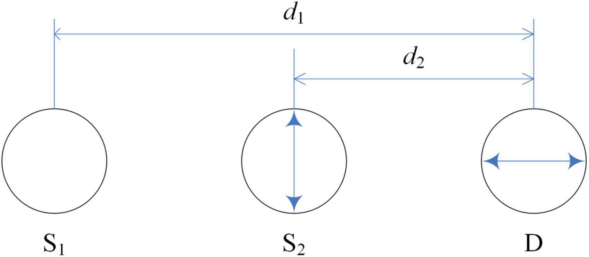
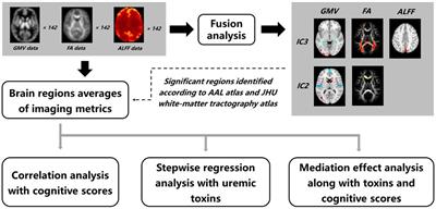
Step 2 is to cancel out the first term because it is independent of the hemodynamic changes. The optode arrangement is depicted in Figure 3. Accordingly, the method assumes that if two unidirectional inline channels have a small distance difference (two sources and one detector), their concentration changes will have similar temporal patterns. The hemodynamic changes contribute to the second term in Eq. (16), so according to the modified Beer–Lambert law, we obtain the following equation:

-log⁡R(n)R(0)=DPF⋅dΔμ(17)

FIGURE 3

Figure 3. Optode arrangement for multidistance optode arrangement technique.

where DPF denotes the differential pathlength factor, d indicates the source-detector distance, and Δμ corresponds to the absorption coefficient change in the gray matter. Moreover, the light transmittances of the source-scalp gaps for both channels and the detector-scalp gap for the detector are denoted by rs1(n), rs2(n), and rd(n), respectively. R1(n) and R2(n) denote the transmittances of the head tissues for the two channels. We can obtain the following equation from Eq. (17) by weighted subtraction of the optical densities of the two channels.

ΔA1(n)-kΔA2(n)=-log⁡rs1(n)rd(n)(rs2(n)rd(n))k

                                                                   -log⁡rs1(0)rd(0)+klog⁡rs2(0)rd(0)

                                                    -log⁡R1(n)R1(0)+klog⁡R2(n)R2(0)

                                      =-log⁡rs1(n)rd(n)(rs2(n)rd(n))k

                                                                                                  +C+(DPF1d1-kDPF2d2)Δμ(n).(18)

The constant k (approximately one) depends on the wavelength, and C is a constant that depends on the initial installation of the device. When the two sources and the detector are fixed relatively well, rs1(n) and rs2(n) will be consolidated to a similar value. Thus, the first term tends to be zero.

The solution above was evaluated on a hairy phantom, and its hardware solution in the first step inspired a creative solution to the hair-blocking problem encountered while using fNIRS devices. The validity of the second step is decided by the approximation that k = 1, whereas in actual measurement, k may occasionally become negative (Yamada et al., 2015). Besides, the optical model neglects detection noise and the angular fluctuation of optodes. The multidistance optode arrangement technique is applied to optical density and is available for real-time monitoring. The solution in Step 1 (using polarized optical film) can attenuate hair-reflected light.

Signal Processing-Based Techniques Wiener filter

The Wiener filter approach is the first to remove motion artifacts without incorporating additional hardware devices (Izzetoglu et al., 2005; Orihuela-Espina et al., 2010; Li L. et al., 2021). The technique assumes that the measured fNIRS signals are a simple addition between the actual fNIRS signals, x(n), and motion artifacts, v(n). Moreover, it is assumed that x(n) and v(n) are stationary and uncorrelated.

corr(x(n),v(n))=0(19)

Consequently, the Wiener filter, g(n), minimizes the mean square error between x(n) and x^(n), that is,

min⁡(E[e(n)2])=min⁡(E[(x(n)-x^(n))2])(20)

Therefore, the optimum filter can be obtained using the orthogonality principle and simplified using Eq. (19) as follows.

corr[e(n),x(n)+v(n)]=corr[x(n),x(n)]

                                                                -g(n)*corr[x(n)+v(n),

                                               x(n)+v(n)]

                                              =0.(21)

We obtain the Fourier transform of the Wiener filter by converting Eq. (21) into the frequency domain using the Fourier transform, which is as follows.

G(w)=px(w)px(w)+pv(w)(22)

where px(w) and pv(w) denote the power spectral densities (PSDs) of the actual fNIRS signals and motion artifacts.

In application, a prior experiment is required to determine the PSDs of g(n) by calculating the values of x(n) and v(n). Subsequently, we can determine g(n) on a time scale using the inverse Fourier transform and apply it to new experimental data.

The Wiener filter is the first attempt to remove motion artifacts without a reference signal from additional hardware devices, such as accelerometers. With the g(n) determined, the filter can be implemented for online applications. However, it requires prior knowledge of the PSDs of x(n) and v(n), which makes initial calibration more complex (a particularly designed paradigm is needed). The idea of building the filter model from a prior experiment inspired later research on motion artifact removal techniques.

Kalman filter

The Kalman filter approach was also proposed based on the general idea of the Wiener filter but as a different model (Izzetoglu et al., 2010). The motion artifact-free fNIRS signal, x(n), was modeled using an autoregressive (AR) model. An AR model of order p can be written as

x(n)=∑i=1paix(n-i)(23)

With the motion artifact-free data from the prior experiment, the parameters of the AR model, ai, i = 1, …, p, can be determined using the Yule-Walker equations. Therefore, the process equation for the Kalman filter has the following form.

ϕ(n)=Aϕ(n-1)+ωn,ϕ(n)=[x(n) ⋯ x(n-p+1)]T(24)

where ϕ(n) is composed of p motion artifact-free fNIRS signals, and ωn denotes the zero-mean noises in the AR model with an error covariance matrix Q. Matrix A can be obtained using Eq. (23) as follows.

A=[a1⋯ap-1ap1⋯00⋮⋯⋯⋮0⋯10](25)

The measurement equation can be written as follows.

z(n)=Cϕ(n)+νn(26)

C=[10⋯0]⏟pelements(27)

where νn denotes the measurement noise (such as the motion artifact) with an error covariance matrix R. z(n) denotes the motion artifact corrupted signal.

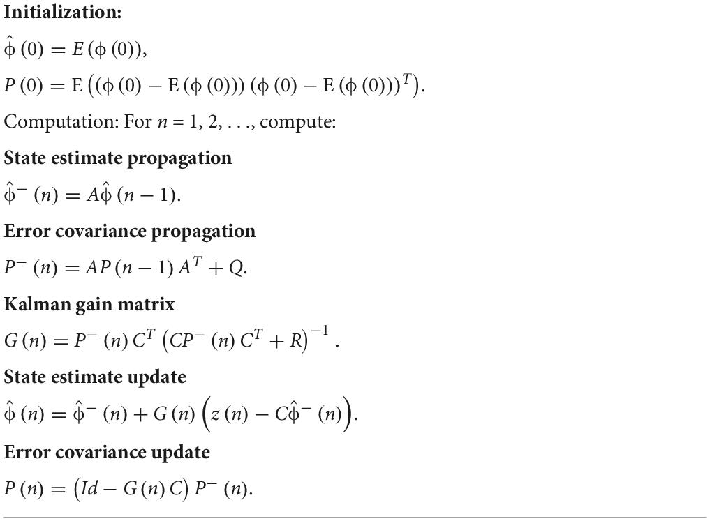
Subsequently, Eqs. (24) and (26) form the state-space model for the Kalman filter, see Table 4. The minus sign in the superscript denotes the prior estimate of a variable. Subsequently, the motion-free fNIRS signal can be obtained using the Kalman filter (Wan and Nelson, 2001). The Kalman filter method can be applied to any online application of optical intensities, optical densities, and concentration changes, and in the Kalman filter theory, both ωn and νn are assumed to be zero-mean Gaussian white noise (Huang and Hong, 2021; Haghighi and Pishkenari, 2021; Li B. A. et al., 2021; Sun and Zhao, 2021; Yang et al., 2021; Lv et al., 2021; Tang et al., 2020; Pham et al., 2021). However, it is not the case for νn (motion artifacts do not observe the zero-mean Gaussian distribution). It may degrade the filter’s performance (Zhou et al., 2017). Moreover, matrices A and C were fixed once determined by the Yule-Walker method. Therefore, further development of the algorithm focuses on; (i) the compensation of the instrumental noises (Amian and Setarehdan, 2013) and (ii) adaptive adjustment of A and C, or using a more sophisticated and nonlinear model in place of Eqs. (24) and (26) (Dong and Jeong, 2018).

TABLE 4

Table 4. Kalman filter algorithm.

Additionally, the state-space model for the Kalman filter method is not unique. A typical example is the incorporation of the autoregressive iterative robust least-squares model (AR-IRLS), the general linear model (GLM), and two linear Kalman filters (Barker et al., 2016). A GLM and an AR-IRLS replaced the state-space model in the Kalman filters. The GLM was introduced to describe the dynamics of hemodynamic responses and physiological noises. The AR-IRLS was introduced as compensation for the MAs in the signals. A difference between the GLM-based method and the AR model-based method is that the GLM-based method requires the information of experimental paradigms, while the AR model-based method does not. Despite the significant adaptation ability of the Kalman filter regarding its state-space model, its applications are limited due to the effort required to set its initial parameters (e.g., the error covariance matrices for the state and the observation).

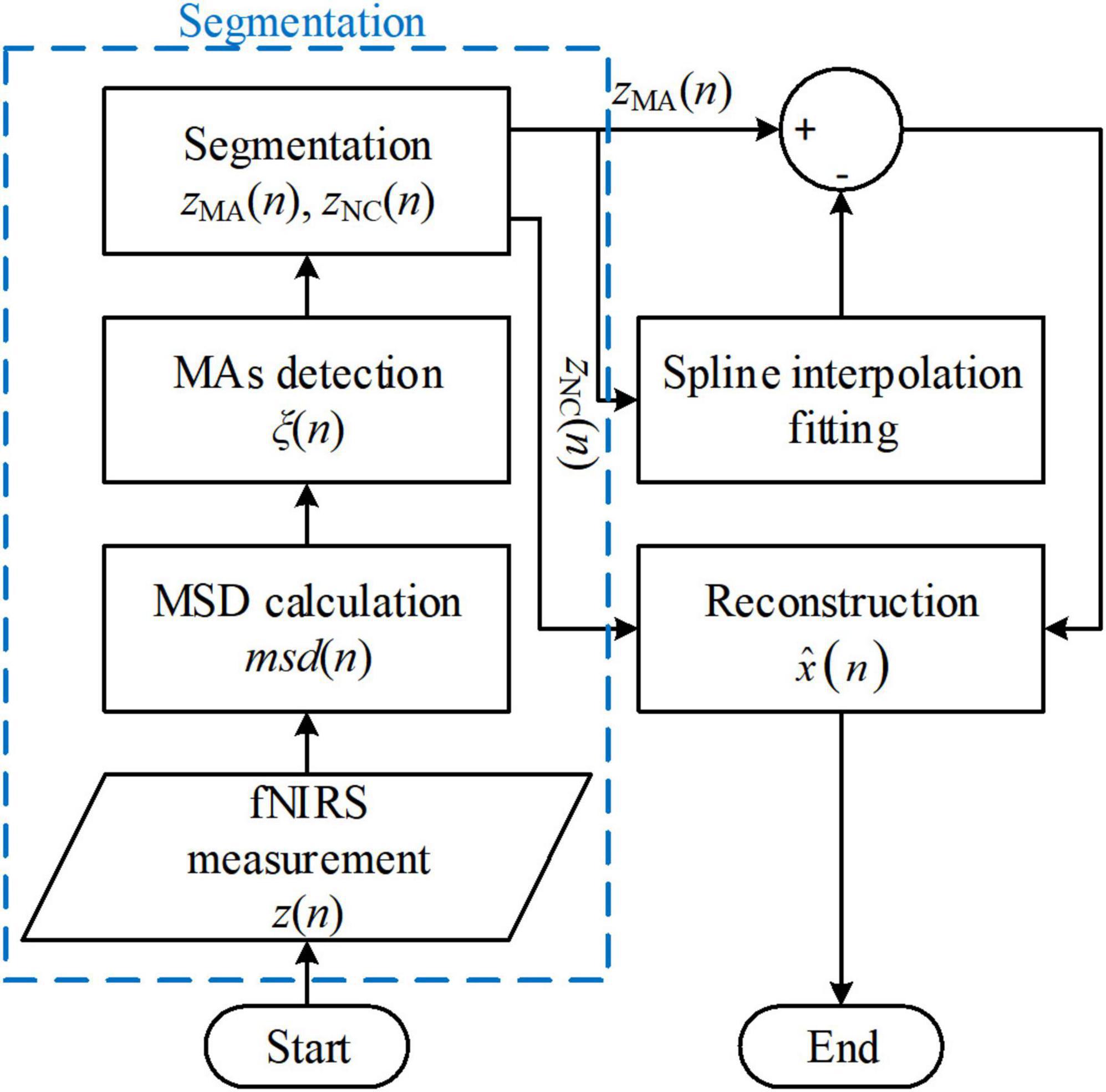
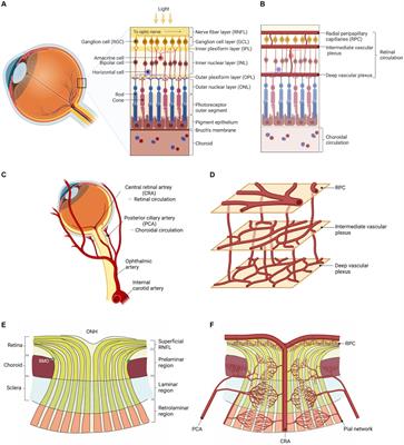
Spline interpolation

The spline interpolation method was first proposed by Scholkmann’s group and is referred to as the MARA (Scholkmann et al., 2010; Selb et al., 2015; Lee et al., 2021). The method made two fundamental assumptions: (i) The measured fNIRS signal is a linear addition of the motion artifacts and the motion-free fNIRS signal, and (ii) in the motion-corrupted segments in the signal, the motion artifact component dominates the measured fNIRS signal. Therefore, the proposed MARA comprised two parts: (i) Motion artifact detection and segmentation, and (ii) motion artifact removal. A flowchart of MARA is illustrated in Figure 4. The spline interpolation method encompasses six processing steps. First, the moving standard deviation (MSD) is calculated within a moving time window of W samples and stored as msd(n).

msd(n)=1W∑i=-kkn+i-1W(∑i=-kkz(n+i))2,W=2k+1,k∈ℕ*(28)

FIGURE 4

Figure 4. Flowchart of the movement artifact reduction algorithm (MARA) algorithm. The process blocks in the blue box are one of the reasons that limit the solution’s online application.

where N* is the set of natural numbers.

We can determine the start and end points of the motion artifacts and store the indices of the corresponding samples in a vector ξ(n) by comparing with the MSD [i.e., msd(n) in Eq. (28)] with a user-defined threshold value T. If the MSD is smaller than T, the corresponding msd(n) will be assigned as zero. The start points and endpoints of motion artifacts can be extracted by considering the first and last samples of non-zero values in msd(n). Next, let us suppose that there are L segments of motion artifacts and let the motion artifact segments, zMA(n), and the non-corrupted segments, zNC(n), be expressed, respectively, as

zMA(n)={zMA,1(n),⋯,zMA,L(n)}(29)

zNC(n)={zNC,1(n),⋯,zNC,L(n)}(30)

Using Eqs. (29) and (30), the measured fNIRS signals can be segmented into non-corrupted segments and motion artifact segments.

In the next part, the spline interpolation method corrects motion artifact segments. Because the motion artifact components dominate the MA segments, the spline interpolation fitting of zMA(n) can be viewed as the motion artifact component. The difference between zMA(n) and its spline interpolation fitting is stored as zdiff(n):

zdiff(n)={zdiff,1(n),⋯,zdiff,L(n)}(31)

Because zNC(n) and zdiff(n) may have different magnitude levels, the final step involves correcting the signal levels for the entire time series. Each segment is parallel-shifted according to the mean of the previous segment and that of the target segment. Two empirical constant thresholds, α = 3–1 Hz–1⋅fs and β = 2 Hz–1⋅fs (where the variable fs denotes the sampling frequency), were chosen for comparison. The detailed shifting rules are listed in Table 1 in Scholkmann et al. (2010).

The spline-interpolation method is used widely for offline analysis in fNIRS studies. It has also been included in some open-source toolboxes, such as HomER2 and NIRSLAB (Balardin et al., 2017). Moreover, the method applies not only to the optical intensities and optical densities but also to concentration changes. However, both the segmentation procedure (the procedures in the blue box in Figure 4) and the parallel-shifting procedure (in the reconstruction process) increase the difficulty for online filtering applications. Moreover, the filter performance depends on artifact detection results (Brigadoi et al., 2014). Some variations of the spline interpolation method have also been proposed (Jahani et al., 2018; Zhou et al., 2021).

Wavelet-based method

The wavelet-based method eradicates motion artifacts by removing the corresponding wavelet coefficients (Molavi and Dumont, 2012; Pinti et al., 2015), without requiring auxiliary devices. The method made the same assumption as the Wiener filter case, that is, z(n) = x(n) + v(n). Based on discrete wavelet transform (DWT), fNIRS signals can be expanded as follows.

z(n)=∑kai0kφi0k(n)+∑i=i0∞∑kbikψ(n)(32)

where i denotes the dilation parameter, k indicates the translation parameter, and i0 denotes the coarsest scale. The scaling function φi0k and the wavelet function ψik are as follows.

φi0k(n)=2i0/2Φ(2i0n-k)(33)

ψik(n)=2i/2Ψ(2in-k)(34)

The