1. Introduction

In recent years, there has been a surge of interest in distributed cooperative control of autonomous surface vehicles (ASVs). It can be envisioned that multiple ASVs enable vehicles to collaborate with each other to execute difficult missions, contributing to improved efficiency and effectiveness over a single one (Arrichiello et al., 2006; Cui et al., 2010; Peng et al., 2011, 2013, 2020, 2021a,b,c; Wang and Han, 2016; Li et al., 2018; Chen et al., 2020; Guo et al., 2020; Liu et al., 2020a,b, 2022; Zhang et al., 2020; Zhu et al., 2021, 2022; Gu et al., 2022a,b,c,d; Hu et al., 2022a,b; Rout et al., 2022). Recently, distributed control methods have been widely studied (see references, Cao and Ren, 2010; Wang et al., 2010; Zhang et al., 2011, 2012; Cui et al., 2012; Zhang and Lewis, 2012; Hong et al., 2013; Peng et al., 2014; Jiang et al., 2021). In Cao and Ren (2010), a distributed control method is proposed to deal with the formation control problem. In Jiang et al. (2021), a distributed model-free control method is designed using a data-driven fuzzy predictor and extended state observers for ASVs to achieve cooperative target enclosing. A distributed adaptive control method is presented to achieve the cooperative tracking with unknown dynamics in Zhang and Lewis (2012). In Cui et al. (2012), a distributed synchronized tracking control method is designed based on an adaptive neural network for ASVs. In Wang et al. (2010), a distributed control approach is designed to deal with the asymptotic tracking under disturbances generated by the exosystem. A distributed leader-follower control method is proposed using the output regulation theory and internal model principle in Hong et al. (2013). In Peng et al. (2014), a distributed adaptive control method is presented by using the state information of neighboring ASVs only. In Zhang et al. (2011), a distributed control method is presented by using the observer to achieve cooperative tracking. In Zhang et al. (2012), an adaptive distributed control technique is designed based on neural network to deal with the cooperative tracking problems. Its key advantage is that the group objective can be achieved via local information exchanges. Consensus-based distributed formation control schemes are presented in Ren (2007), Ren and Sorensen (2008), and Hu (2012). In Ren (2007), a consensus-based distributed control method is proposed to deal with the formation control problem. In Ren and Sorensen (2008), a consensus-based approach is designed to achieve the distributed formation control. In Hu (2012), a distributed consensus-based control method is designed to achieve global asymptotic consensus tracking.

As for autonomous surface vehicle systems, the modeling process is time-consuming and a large number of experiments is required for identifying model parameters. On the other hand, robustness against model uncertainty and ocean disturbances is critical for high-performance control of ASVs (Fossen, 2002; Skjetne et al., 2005; Tee and Ge, 2006; Li et al., 2008; Dai et al., 2012; Chen et al., 2013; How et al., 2013). To deal with this problem, adaptive backstepping and DSC techniques has been widely suggested; see the references (Fossen, 2002; Skjetne et al., 2005; Tee and Ge, 2006; Li et al., 2008; Dai et al., 2012; Chen et al., 2013; How et al., 2013). In Tee and Ge (2006), a stable tracking control method is proposed using backstepping and Lyapunov synthesis for multiple marine vehicles under the unmeasurable states. In Chen et al. (2013), a variable control structure based on backstepping and Lyapunov synthesis is designed for the positioning of marine vessels with the parametric uncertainties and ocean disturbances. In How et al. (2013), an adaptive approximation technique is designed using the backstepping to estimate the uncertainties. In Dai et al. (2012), an adaptive neural networks control method is designed based on the backstepping and Lyapunov synthesis with uncertain environment. In Skjetne et al. (2005), an adaptive recursive control method is designed using the backstepping and Lyapunov synthesis for marine vehicles with the unknown model parameters. Although the adaptive backstepping and DSC are recursive and systematic design methods, it does not offer the freedom to choose the parameter adaptive laws (Krstić et al., 1995). Besides, the identification process depends on the tracking error dynamics, and the transient performance cannot be guaranteed (Cao and Hovakimyan, 2007; Yucelen and Haddad, 2013).

Motivated by the above observations, this article presents a distributed constant bearing guidance and model-free disturbance rejection control method for formation tracking of ASVs subject to fully unknown kinetic model. Specifically, a distributed constant bearing guidance law is designed at the kinematic level to achieve a consensus task. Then, an AESO is constructed for estimating the model uncertainty and unknown ocean disturbances, which can achieve the uncertainty and disturbance estimation. Next, a controller module is developed by using a DSC technique. Simulation results are provided to show the efficacy of the proposed modular design integrated distributed constant bearing guidance and model-free disturbance rejection control method. The main contribution of the proposed control method are stated as follows. Firstly, the proposed design results in the decoupled estimation and control, where the estimation loop is faster than the control loop, yielding the improved transient performance. This contributes to the certainty equivalence control of multi-vehicle systems. Secondly, the security level of ASVs is enhanced by using an AESO to identify the total uncertainties. Finally, the salient feature of the proposed method is that a cooperative behavior can be achieved without knowing any priori information.

The rest of this paper is organized as follows: The problem formulation is presented in Section 2. Section 3 presents the distributed constant bearing guidance and model-free disturbance rejection control method. Section 4 provides simulation results to illustrate the designed model-free disturbance rejection control method for distributed formation tracking. Section 5 concludes this paper.

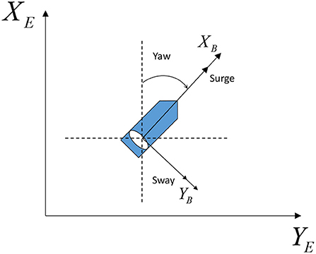
2. Problem formulation

A three degree-of-freedom (DOF) dynamical model for ASVs in a horizontal plane as shown in Figure 1 can be expressed with kinematics (Fossen, 2002; Skjetne et al., 2005).

η·i=R(ψi)νi,    (1) ν·i=Mi-1fi(νi)+Mi-1τi+Mi-1τwi(t),    (2)

where

R(ψi)=[cosψi-sinψi0sinψicosψi0001] ;    (3)

ηi=[xi,yi,ψi]T∈ℝ3 represents the earth-fixed position and heading; νi=[ui,vi,ri]T∈ℝ3 includes the body-fixed surge and sway velocities, and the yaw rate; Mi=MiT∈ℝ3×3,Ci(νi)∈ℝ3×3,Di(νi)∈ℝ3×3 denote the inertia matrix, coriolis/centripetal matrix, and damping matrix, respectively; τi=[τui,τvi,τri]T∈ℝ3 denotes the control input; τwi(t)=[τwui(t),τwvi(t),τwri(t)]T∈ℝ3 represents the disturbance vector caused by the wind, waves, and ocean currents.

FIGURE 1

Figure 1. The plane motion diagram of the ASV.

Since the robot dynamics (1) contain unknown dynamics induced by model uncertainty and ocean disturbances, we rewrite the robot kinetics (1) as follows.

η·i=R(ψi)νi,    (4) ν·i=Λiτi+si,    (5)

where

si=Mi-1fi(νi)+Mi-1τwi(t),Λi=Mi-1.    (6)

The control objective is to design a cooperative control law τi for ASVs with dynamics (1) to track a reference trajectory η0(t) such that

limt→∞||ηi(t)-η0(t)||≤δi,    (7)

for some small constant δi.

We use the following assumption.

Assumption 1: The reference signals η0(t), η·0(t), and η¨0(t) are bounded.

3. Cooperative tracking

In this section, a modular design approach is presented to develop the cooperative formation controllers for ASVs. First, by using the designed AESO to estimate the total uncertainties and fully unknown input coefficients, a simplified model-free dynamic kinematic controller is designed with the aid of a dynamic surface control.

3.1. Controller design

Step 1. At first, a cooperative tracking error is defined as

zi1=RiT{∑j∈Niaij(ηi−ηj)+ai0(ηi−η0)},    (8)

where RiT=RT(ψi), and aij and ai0 are determined by the communication graph, if the ith ASV obtains the information of the jth, aij = 1; otherwise, aij = 0. The definition of ai0 is similar to aij.

Assumption 2: The augmented graph contains a spanning tree with the root node being the leader node n0.

Then, define a global formation tracking error ϵi as

Define L as the Laplacian matrix of the graph and A0 as the leader adjacency matrix, which leads to

z1=R(H⊗I3)ϵ.    (10)

where H=L+A0, z1=[zi1T,...,ziNT]T, ϵ=[ϵ1T,...,ϵNT]T, and R=diag. Define aid = di + ai0, then, it follows from (1) that the time derivative of zi1 in (8) is obtained

żi1=-riSzi1+aidνi-∑j∈NiaijRiTRjνj-ai0RiTη·0,    (11)

where

S=[0-10100000].    (12)

A distributed constant-bearing guidance law αi1 is proposed as follows

αi1=1aid{−kiηzi1zi12+Δ2+∑j∈NiaijRiTRjνj+ai0RiTη˙0},    (13)

where Δ is positive constant, and kiη=diag∈ℝ3×3 with kiη1 ∈ ℝ, kiη2 ∈ ℝ, and kiη3 ∈ ℝ being positive constants.

Let us suppose here that αi1 are unknown, and let it pass through a first-order filter as follows

γiν·id=αi1-νid,νid(0)=αi1(0),    (14)

where γi ∈ ℝ.

Then, the derivative of qi is obtained as

q·i=-qiγi-α·i1.    (15)

where qi = αi1 − νid.

Now using (15), we can conclude that

qi(t)=qi(0)e-tγi-∫0te-1γi(t-τ)α·i1(τ)dτ.    (16)

We can obtain that the bound of ||qi(t)|| satisfies the following inequality

||qi(t)||≤||qi(0)||e-tγi+αi1*γi,

where αi1* is a positive constant.

Step 2: To start with, define the velocity tracking error zi2 as

zi2=νi-νid.    (17)

Take the time derivative of zi2 along (4) is

z·i2=Λiτi+si-ν·id.    (18)

For the robot kinetics (4), an AESO is designed as

∈ℝ3×3,kis=diag∈ℝ3×3, and kiν1 ∈ ℝ, kiν2 ∈ ℝ, kiν3 ∈ ℝ, kis1 ∈ ℝ, kis2 ∈ ℝ, and kis3 ∈ ℝ are positive constants. ν^i, ŝi, σ^i, and Λ^i are the estimates of νi, si, σi, and Λi, respectively.

Assumption 3: For unknown functions si and σi, there are si*∈ℜ+ and σi*∈ℜ+, such that ||ṡi||≤si* and ||σ·i||≤σi*.

Let the parameter estimation be Λ~i=Λ^i-Λi, and the prediction error be ν~i=ν^i-νi. Define s~i=ŝi-si and σ~i=σ^i-σi. It can be obtained σ^i-Λ^iτi=-s~i-Λ~iτi+ai1 with ai being the reconstruct error. Then, the error dynamics can be expressed as

∈ℝ3×3, and kiτ1∈ℝ+,kiτ2∈ℝ+, and kiτ3∈ℝ+.

Substituting (21) into (18) yields

Miz^·i2=-kiτz^i2-ϱiν~i,    (22)

where ϱi is a positive constant.

The following lemma presents the stability of AESO error subsystem (20).

Lemma 1: Under Assumption 2, the AESO error subsystem (20), viewed as a system with the states being ν~i, s~i, σ~i, and Λ~i, the inputs being ṡi, σ·i, and Λ·i is ISS.

Proof : Construct the Lyapunov function as

Vσi=12(σ~iTΓσi-1σ~i+Λ~iTΓΛi-1Λ~i),    (23)

and the time derivatives of Vσi is

V·σi=σ~iΓσi-1(-Γσi(ŝ