Introduction

In recent years, online social media and mobile smart terminals have emerged in large numbers and developed rapidly. They provide people with new communication process and interactive spaces, making people's lifestyles change dramatically (Aprem and Krishnamurthy, 2017). A growing number of people tend to use smart terminals to obtain information, exchange ideas and spread information through online social media. The process of information dissemination is no longer the one-way communication of traditional media, but interactive communication (Nduhura and Prieler, 2017). Among them, there is a large amount of text as the simplest and most direct carrier for human beings to express their thoughts and spread knowledge in the Internet. It involves hot events, product reviews, news information and many other aspects. They contain rich emotional information and attitudinal views, with high social value and commercial application value (Liu et al., 2017). Emotion, a physiological and psychological state that results from a combination of feelings, thoughts, and behaviors (Chao et al., 2017). Such as happiness, sadness and anger are also among the chief factors that influence human behavior. People discuss certain hot topics and express their opinions on social platforms. They publish reviews of products or services on shopping platforms, etc. These unstructured online texts contain a lot of valuable information about users' emotions (Angioli et al., 2019). These emotional messages inherently have a certain abstraction and are difficult to be processed directly. It has attracted the attention of many researchers to find out how to extract this effective information from the huge amount of web texts and then apply it effectively in real life, resulting in the emergence of dynamic user text sentiment analysis techniques.

Initial studies on sentiment analysis focused on coarse-grained research on sentiment polarity dichotomization or trichotomization. With the gradual research on text sentiment analysis techniques and the desire to have a more comprehensive understanding of users' psychological states, the study of text sentiment analysis gradually shifted to more fine-grained multi-categorization research. Emotion recognition is the foundation and prerequisite of emotion classification. In the vast amount of realistic web texts, there are filled with abundant unemotional texts and emotional texts. Emotionless text is an objective description of things or events without any emotion. Emotional texts contain personal emotions such as happiness, anger, sadness and so on. Emotional texts are the main object of textual emotion analysis, therefore, it is necessary and chief to identify the presence or absence of emotions in a large amount of real texts and filter out emotional texts. Sachdev et al. (2020) collected a corpus of blog posts, which were annotated with word-level emotion categories and intensities, and used a knowledge-based approach to identify sentences with and without emotions with an accuracy of 73.89%. Wallgrün et al. (2017) constructed a corpus oriented to microblogging texts, annotated whether the microblogging texts contain emotion information or not. At the same time, they performed a multi-label annotation of the emotion categories contained in the microblog texts with emotions. They summarized the results of the NLP&CC2013 Chinese microblog sentiment analysis evaluation task on sentiment recognition, which facilitated the research related to sentiment analysis. Huang et al. (2017) planned a text emotion recognition process based on syntactic information, which expands the performance of emotion recognition by making full use of syntactic information through lexical annotation sequences and syntactic trees. Emotion classification, as chief research direction of emotion analysis, is based on emotion recognition to classify texts containing emotion information at a finer granularity and obtain the specific emotion category (e.g., happy, angry, sad, etc.) expressed by the user in the text. The majority of early sentiment classification studies utilized lexicon- and rule-based process to determine sentiment categories. Fine-grained multi-class sentiment classification is the difficulty and focus of sentiment analysis, researchers have studied sentiment classification from different perspectives, such as construction of sentiment corpus (Fraser and Liu, 2014; Kawaf and Tagg, 2017), author sentiment and reader sentiment prediction (Chang et al., 2015; Yoo et al., 2018), document-level sentimentality organization, sentence-level sentimentality organization and word-level sentiment classification (Liu et al., 2020; Zhang, L., et al., 2021). Alves and Pedrosa (2018) planned a process based on frequency and co-occurrence information to classify the sentiment of headline texts by making full use of the co-occurrence relationship between contextual words and sentiment keywords. Subsequently, various researchers have used traditional machine learning-based process for sentiment classification studies. Pan et al. (2017) planned a multi-label K-nearest neighbor (KNN) based sentiment classification process that explores the polarity of words, sentence subject-verb-object components, and semantic frames as features for their impact on sentiment classification. To differ from this, Aguado et al. (2019) have taken into accounts the interaction of sentiments between sentences and use a coarse-to-fine analysis strategy to do sentiment classification of sentences, first obtaining the set of possible sentiments embedded in the target sentence roughly using a multi-label K-nearest neighbor approach, and then refining the sentiment category of the target sentence by combining the sentiment transfer probabilities of neighboring sentences. Rao et al. (2016) utilized a maximum entropy model to model words and multiple sentiment categories in a text to estimate the relationship between words and sentiment categories to classify sentiment in short texts. Traditional machine learning process extract text features manually through feature engineering, while deep learning uses representation learning process to extract text features automatically without relying on artificial features. Effective feature extraction is the core of research on emotion classification process, and most of research works show that reasonable use of deep learning techniques based on neural networks to extract rich semantic information in emotional texts contributes to the effectiveness of text emotion classification. Abdul-Mageed and Ungar (2017) constructed a large-scale fine-grained sentiment analysis dataset employing Twitter data and designed a represent neural network based on gating units to achieve 24 classes of fine-grained sentiment classification. Kim and Huynh (2017) experimentally explored text emotion classification utilizing the LSTM model as well as its variant nested long-short-term memory network (Nested LSTM) model, respectively, which showed that the Nested LSTM model facilitates better accuracy of sentiment classification. Wang et al. (2016) planned neural network (NN) model based on bilingual attentively mechanisms for the problem of emotion classification in bilingual mixed text, where the LSTM model is used to construct a document-level text illustration and the attention mechanism captures semantically rich words in both monolingual and bilingual texts. In addition, some studies have applied a joint multi-task learning approach to the task of emotion classification. Awal et al. (2021) incorporated emotion classification and emotion cause detection as two subtasks into a unified framework through a joint learning model, trained simultaneously to extract the emotional features needed for emotion classification and the event features needed for emotion cause detection. Yu et al. (2018) planned a dual-attention-based transfer learning process that aims to improve the performance of emotion classification using sentiment classification. At present, there are plenty of results for research on text sentiment analysis process, but sentiment analysis still faces many challenges due to the colloquial and irregular nature of online texts and the complexity of sentiment itself (Ning et al., 2021). For text representation, most approaches use pre-trained models such as Word2Vec and GloVe to obtain word directions, which are simple, efficient, and can characterize contextual semantics well, but suffer from the problem of multiple meanings of a word (Ning et al., 2022). For text feature extraction, commonly used NNs such as CNN and Bi-LSTM extract semantic features while ignoring the syntactic hierarchy features of the text (Ning et al., 2020). Most approaches only symbolize sentiment category labels and act as a supervisory role in the classification process, while ignoring semantic information contained in the labels themselves, which is undoubtedly a “semantic waste”. In this paper, we explore and improve the text sentiment analysis process based on the above three problems.

Based on this, the main research of this paper is to use deep learning techniques to accomplish the task of emotional analysis of online text, based on the ordered neuronal long and short term memory network (ON-LSTM) and attention mechanism, and incorporating the semantic information of emotional category labels to build the emotional analysis model ON- LSTM-LS. First, the text features are extracted based on ON-LSTM and attention mechanism. Then the sentiment analysis model based on ON-LSTM and label semantics. In this study, for online social text, we build the sentiment analysis model ON-LSTM-LS based on ordered neuron long and short term memory network and attention mechanism, and incorporate the semantic information of sentiment category labels to improve the performance of text sentiment analysis.

Theory and model construction Text representation

Text data usually consists of a set of unstructured or semi-structured strings. Since computers cannot directly recognize and process text strings, they need to numerate or directionize the text, i.e., text representation. Text representation enables computers to process real text efficiently and is a fundamental and chief step in the study of text sentiment analysis. In Chinese, words are generally considered to be the most basic semantic units of text. Therefore, general research for Chinese text should first perform word separation operation, and then the words in the text are represented afterwards.

Word direction representation

NN-based distributed representation is also recognized as word direction, word embedding or distributed representation of words. This process models the target word, context of target word and the relationship between them, and represents the target word as a low-dimensional solid real-valued direction in continuous space. Compared with matrix-based distributed representation and cluster-based distributed representation, word direction representation can contain more and more complex semantic information. It is extensively used in various normal language dispensation errands.

The word directions are gained by training the language model, which uses a single-layer NN to perform the solution of the binary language model while obtaining the word direction representation. Based on this, the NN language model NNLM is planned (Wang et al., 2022). The model takes the first k words of the present word wt, wt−k−1, …, wt−1, as input and uses a NN to predict the conditional likelihood of the occurrence of the present word wt to obtain a word direction representation while training the language model. As the NNLM is capable of handling only fixed-length sequences, lacking flexibility. Due to the slow training speed, the researchers improved the NNLM. They planned two words direction training models, which are successive bag-of-words model CBOW and skip-word model. They open source a tool Word2Vec for word direction computation. Differs from the NNLM in which the representation of the present word wt depends on its predecessor. In CBOW and Skip-gram models, the representation of the present word wt depends on k words before and after it. In the CBOW and Skip-gram models, representation of present word wt depends on k words before and after it.

Both CBOW and Skip-gram models have same three-layer hierarchy: input layer, mapping layer, output layer, and structure diagram are exposed in Figure 1A. In the input layer, the input words are randomly initialized as N-dimensional directions. They enter the hidden layer after a simple linear operation, and then likelihood distribution of the target words is output by hierarchical Softmax.

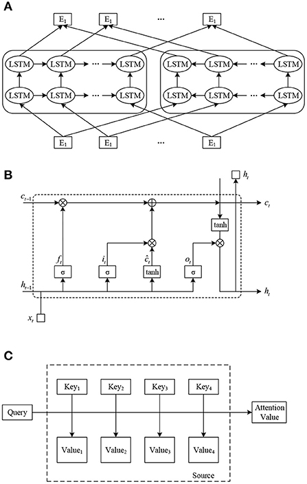
FIGURE 1

Figure 1. Model structure diagram. (A) ELMo model structure diagram. (B) LSTM model structure diagram. (C) Attention model structure diagram.

The CBOW model is to predict the provisional likelihood of the occurrence of the word wt by the context of present word wt, which is calculated as:

p(wt|ct)=exp(e′(wt)Tx)∑i=1|V|exp(e′(wi)Tx)    (1) x=∑i∈ke(wi)    (2)

where ct denotes the words in the context window, e(wt) is input direction of word wt, e′(wt) is output direction of word wt, x is the context direction, V is the corpus word list.

The Skip-gram model uses the present word wt to predict the conditional likelihood of each word in the vocabulary to occur in its context (Wang et al., 2021) and is calculated as:

p(wj|wt)=exp(e′(wj)Te(wt))∑i=1|V|exp(e′(wi)Te(wt))    (3)

To limit the number of restrictions to restore the training efficiency of the model, Word2Vec is optimized using two techniques, hierarchical Softmax and negative sampling. In the training process of model, representation of words is constantly updated by the output direction of the mapping layer is the direction of words.

Considering that Word2Vec only considers contextual co-occurrence features within a finite window when learning, global statistical features are ignored. Researchers propose the GloVe word embedding technique that fuses global and local contextual features of text. gloVe belongs to matrix-based distribution representation, which is a global logarithmic bilinear regression model. They construct global word-word co-occurrence matrices based on the statistical information between words in the corpus. They use a global matrix decomposition and local context window approach for unsupervised training of non-zero positions in the co-occurrence matrix, and a back-propagation algorithm to solve the word directions. Compared with Word2Vec, GloVe has stronger scalability.

Word2Vec and GloVe use pre-training techniques to represent each word as a word direction with a contextual semantic representation. They solve the problems of sparse data, dimensional disaster, and lack of semantic information representation that exist in traditional one-hot directions. At the same time, they have become the mainstream text representation techniques because of their simplicity and efficiency. They have greatly contributed to the development of natural language processing research.

Dynamic word direction technique

While the word direction representation techniques, represented by Word2Vec and GloVe, have greatly advanced the development of natural language processing, they also have some problems. One of the biggest problems is polysemy. Word2Vec and GloVe learn word directions as static word directions, i.e., the word-direction relationship is one-to-one. In other words, no matter how the context of a word changes, the trained word direction is uniquely determined and does not change in any way as the context changes. This static word direction cannot solve the problem of multiple meanings of a word. To solve the problem, researchers have conducted some exploratory research. They have planned a dynamic word direction technique based on language model. Dynamic word directions are not fixed, but change at any time according to the contextual background. ELMo, a language model that can be used to train dynamic word directions, is presented next.

ELMo (Embedding from Language Models) is a novel deep contextualized word representation model planned by Peters et al. By training the model, high quality dynamic word directions can be gained. The model is trained using a deep bi-directional language model (biLM) to obtain different word representations for different contextual inputs, i.e., to generate word directions dynamically.

ELMo uses a two-stage training process. The first stage is to pre-train a language model on a large corpus using a multilayer biLM before training on a specific task. This language model is equivalent to a “dynamic word direction generator” that generates specific word directions for a specific task. In the second stage, the word directions generated by the language model in the first stage are added to the downstream task as a feature supplement for task-specific training. The model structure of ELMo is exposed in Figure 1B. Where (E1, E2, …, EN) are the static Word Embedding of the input word sequence, (T1, T2, …, TN) are the dynamic Word Embedding of the output gained by pre-training the ELMo model.

The ELMo model employs bivectorial LSTM language model to train word representation in the first stage. Specifically, suppose that given a word sequence (w1, w2, …, wN) of length N, the forward LSTM language model calculates the sequence likelihood of the occurrence of the word at the 1, 2, …, k−1 by taking the word sequence at the given first position as:

p(w1,w2,…,wN)=∏k=1Np(wk|w1,w2,…,wk-1)    (4)

The backward LSTM language model calculates the sequence likelihood of the occurrence of words at position k + 1, k + 2, …, k + N by taking the sequence of words at position k given as:

p(w1,w2,…,wN)=∏k=1Np(wk|wk+1,wk+2,…,wN)    (5)

The combination of frontward LSTM language model and backward LSTM language model constitutes the bi-directional language model biLM, which is required to maximize the following objective function during the training process as:

∑k=1N(logp(wk|w1,w2,…,wk-1;Θx,Θ→lstm,Θs)+logp(wk|wk+1,wk+2,…,wN;Θx,Θ←lstm,Θs))    (6)

where Θx denotes the word direction matrix, Θx is the parameter of the softmax layer, Θ→lstm and Θ̄lstm denote frontward LSTM language model and the backward LSTM language model, respectively.

The L-layer biLM model is used in the pre-training, and the word representations gained from each layer have different features. For each input word, the word representation with features such as syntactic semantics is output for it by pre-training with the L-layer biLM model as:

Rk=     =    (7)

where hk,0LM is the word layer, hk,jLM=|h→k,jLM,h←k,jLM|.

A language model and word representations for each hidden layer will be gained after the first stage of training. In the second stage, the sentences in the downstream task will be used as input to the dimensional ELMo. For each word in the sentence, ELMo combines the word representations of all hidden layers into a direction by calculating the weights of each hidden layer. That is, a direction of words in the present context. It is formalized as:

ELMoktask=E(Rk;Θtask)=γtask∑j=0Lsjtaskhk,jLM    (8)

where γtask is the validated global scaling factor and sjtask is the softmax normalized weighting factor.

ELMo is able to dynamically generate different word directions for the similar word in dissimilar circumstances. It conforms to the word direction of the present context. It solves the problem of encoding multiple meanings of a word to some extent and performs well in several natural language processing tasks.

Deep learning models

The concept of deep learning (DL) (Wang et al., 2021) originated from the study of artificial NNs. It involves of multiple layers of artificial NNs connected to be able to extract effective feature representation information from a large amount of input data. Deep learning mimics the way the human brain operates. It learns from experience and has the ability to excel in representation learning. It has been successfully applied in several research fields.

Represent NNs

Represent neural network (RNN) is a NN with short-term memory capability to process temporal information of varying lengths. It is widely used for several tasks in natural language processing. RNNs use neurons with self-feedback to process temporal information of arbitrary length by unfolding multiple times. Where xt denotes input direction at the time of t, ht denotes state of the hidden layer at the time of t. ot denotes output direction at the time of t. U denotes Input layer to hidden layer weight matrix, V denotes Value matrix of weights from hidden layer to output layer. W denotes value of the weight matrix of the preceding moment of hidden layer as input value of the current moment.

The RNN gives an output ot with present network hidden layer state ht for input xt at t. The value of ht at time t depends upon not only xt, as well as also on the hidden layer state ht−1 at previous moment, calculated as:

ht=f(Uxt+Wht-1)    (10)

where f represents a non-Linear activation function such as sigmod or tanh. The network parameters are shared at different moments and are trained by the backpropagation over time algorithm (BPTT).

Theoretically, RNNs are capable of handling text sequences of arbitrary length. However, in practice, when the length of text sequences is too long, the problem of gradient explosion or gradient dispersion occurs. It makes parameter updating difficult, which in turn prevents RNNs from learning long-range dependency information. It also leads to biased learning results of long-range dependencies, i.e., RNNs learn short-term dependence.

Short long-term memory network

A variation of RNN, Long-Short-Term Memory Network (LSTM) can effectively tackle the problem of gradient explosion or gradient dispersion in RNN (Yan et al., 2021). The improvement of LSTM for RNN is twofold. On the one hand, during the training process of the network, RNN has only one state ht at the moment t, LSTM adds a state ct on this basis, ct represents the memory state of the represent unit, which involves a small number of function operations and thus can store long distance information. On the other hand, LSTM introduces a gating mechanism and designs three gate structures, forgetting gate, input gate, and output gate, which enable represent NN to selectively forget some unchief information while remembering the past information through the interaction between the three gates, and thus learn longer distance dependencies.

The cell of LSTM has certain memory function because of it. It also called a memory cell. The structure of the LSTM loop cell is exposed in Figure 1B. where xt represents input direction of the memory cell at moment t. ht represents output direction of the memory cell at time t. represents present information after updating the memory. ft, ot and it represent the forgetting gate, output gate and input gate, respectively.

The forgetting gate ft selectively forgets a portion of the cell state information through the sigmod layer, i.e., it determines how much of the cell condition ct−1 of previous moment needs to be retained in the cell state ct of the present moment. The calculation formula is as follows:

ft=σ(Wfxt+Ufht-1+bf)    (11)

Input gate it selectively records new inputs in the memory cells through the sigmod layer. It determines how much of the present network's input xt needs to be saved into the cell state ct. Also, the cell state ct of the present input is determined based on the output ht−1 of hidden layer state and xt at the present moment, which is calculated as follows:

it=σ(Wixt+Uiht-1+bi)    (12) ĉt=tanh(Wcxt+Ucht-1+bc)    (13)

The present memory ĉt and the historical memory ct−1 need to be combined before the output gate to update the cell state ct at the present moment. The forgetting gate allows chief information from long ago to be preserved, and the input gate allows irrelevant information from the present input to be filtered and forgotten.

ft=σ(Wfxt+Ufht-1+bf)    (14)

The output gate ot inputs the input information and the present cell state update to the next hidden layer ht through the sigmod layer, i.e., it controls how much of the cell state ct needs to be output to the hidden layer state ht at the present moment. The calculation formula is as follows:

ot=σ(Woxt+Uoht-1+bo)    (15) ht=ot◦tanh(ct)    (16)

In the above equations, Wf, Wi and W◦ are weight matrices from input layer to the forgetting gate, input gate and output gate, respectively. Uf, Ui and Uo are weight matrices from output layer to the forgetting gate, input gate and output gate, respectively. Wc is connection weight from input layer to the LSTM loop unit. Uc is the connection weight from the previous node to the present node of the LSTM loop unit, bf, bi, bo and bc are all offsets.

Weight parameters in RNN are shared across time steps, which is why there is gradient explosion or dispersion. In contrast, there are multiple paths of gradient propagation in LSTM. In which the process of cell state update at the present moment is carried out by element-by-element multiplication and summation. Its gradient flow is relatively stable, thus greatly reducing the risk of gradient explosion or dispersion. Thus, LSTM is able to handle long-range temporal information.

The input gate determines degree of retention of the input information. The forgetting gate determines the extent to which memory information is forgotten. The output gate, on the other hand, controls the extent to which internal memory is output to the outside. Each of the three gating switches has its own role, which enables LSTM to effectively use historical information and establish long-range temporal dependencies. In turn, it is widely used in tasks related to sequential problems.

Gated circulation unit

Gated represent unit (GRU) is a represent NN based on another gating mechanism. The basic design idea of GRU is the same as LSTM, and it can be said to be a variant of LSTM. Its difference lies in two main aspects. On the one hand, the structure of GRU is relatively simple, using two gate structures. The reset gate determines how much historical information requires to be forgotten. The update gate determines how much of the history information can be saved to the present state. On the other hand, GRU directly passes the hidden state to the next cyclic unit without using an output gate.

Where xt represents input direction at the present moment, ht−1 represents state at previous moment, h~t is the candidate state at the present moment, rt and zt represent reset gate and update gate, respectively, and output direction ht at the present moment is calculated as in Eqs. (17–20).

rt=σ(Wrxt+Urht-1)    (17) zt=σ(Wzxt+Uzh