Introduction

Autism spectrum disorder (ASD) is a neurodevelopmental disorder characterized by early deficits in social interactions and communication and restricted and repetitive activities and interests (American Psychiatric Association, 2013). As its name suggests, rather than a single condition, ASD includes a wide range of symptoms (Tanu and Kakkar, 2019) that reflect an overarching diagnostic category that, before the fifth edition of the Diagnostic and Statistical Manual of Mental Disorders (DSM-5), was comprised of multiple separate disorders, such as Autistic disorder, Asperger’s syndrome, and other pervasive developmental disorders (American Psychiatric Association, 2013). Language difficulties, epilepsy, and other problems may come with ASD (Yasuhara, 2010; Sivapalan and Aitchison, 2014). The prevalence of ASD in the United States has grown from 1 in 110 to 1 in 69 over 4 years (from 2008 to 2012) (Lee and Meadan, 2021). Approximately 1% of the world’s population was diagnosed with ASD, and its prevalence among males is four times higher than among females (World Health Organization, 2013; Gao K. et al., 2021). ASD’s etiology is still elusive, but genetics and the environment may play a role (Chaddad et al., 2017).

Early diagnosis and effective intervention improve the quality of life for autistic individuals (Pagnozzi et al., 2018). The gold standard for diagnosing most mental disorders, including ASD, is observation and visual analysis of behavior, such as interviews (Zhang L. et al., 2020; Jarraya et al., 2021). These instruments, however, have limits. A child’s apparent inability to cope with their environment is usually diagnosed at 3 years old (Wang et al., 2018). Interpretive coding of children’s observations is time-consuming (Eslami et al., 2021). Comorbidities and other disorders that share prominent features with ASD may hinder diagnostic evaluation (Gargaro et al., 2011). Clinical training, tools, and cultural context may influence a clinician’s subjective observations (Eslami et al., 2021). These limitations necessitate more optimal diagnosis methods, such as biomarker-based diagnosis.

In the 1990s, MRI techniques such as structural MRI (sMRI) and functional MRI (fMRI) evolved significantly (Libero et al., 2015; Eslami et al., 2021). Each modality gives unique information about the brain (Ozonoff et al., 2011; Wang et al., 2018). sMRI can dissect brain structures in different images, such as T1 and T2 weighted, and T2-weighted Fluid Attenuated Inversion Recovery (FLAIR) (Mostapha, 2020; Eslami et al., 2021). sMRI also tracks brain growth over time in longitudinal studies, showing early life risk factors (Li et al., 2019a). fMRI tracks changes in blood flow to brain regions that stimulate neurons (Mostapha, 2020). The two main forms of fMRI are rs-fMRI and task fMRI (Xu et al., 2021).

Numerous studies have explored brain abnormalities in the cerebellum (Sivapalan and Aitchison, 2014), gray matter (GM) volumes (Rojas et al., 2006), and brain functional connectivity (FC) (Nomi and Uddin, 2015), and others using statistical methods (Polsek et al., 2011). However, the interdependency between diverse brain regions has been neglected (Libero et al., 2015; Eslami et al., 2021). In addition, group differences are not individual differences, so results from research cannot be directly translated into clinical practice (Rojas et al., 2006; Xu et al., 2021). Machine learning (ML) models and deep learning (DL) techniques have recently become attractive to be applied in the diagnosis of diseases like Parkinson’s (Manzanera et al., 2019) and epilepsy (Abbasi and Goldenholz, 2019). Conventional ML methods facilitate the exploration of complex abnormal imaging patterns and consider the relationships between different brain regions (Xu et al., 2021). Thus, it can greatly enhance the role of statistical methods. Computer-aided diagnostic (CAD) systems are also a low-cost method that reduces healthcare expenditure compared with other methods. They’re simple enough that even computer scientists with no prior training in psychiatry can analyze data and extract insights (Manzanera et al., 2019; Eslami et al., 2021). In ML, the key features are usually extracted manually and then tell the algorithm how to make a prediction or classification by consuming more information. For problems with complex nonlinear relationships, the DL algorithm is better suited because it learns features automatically and its performance is superior in image analysis fields, such as object detection and image classification (Zhang et al., 2021). However, the diagnosis of ASD remains a formidable challenge, as studies based on ML have shown different results that may reflect the diversity of behavioral symptoms of the disorder and its proposed etiology, often linked to the brain (Sivapalan and Aitchison, 2014).

Several publications (Zhang L. et al., 2020; Zhang et al., 2021; Quaak et al., 2021) have reviewed the classification of ASD using only ML or DL algorithms. Some representative examples of previous reviews are listed in Table 1.

TABLE 1

Table 1. ASD application review papers based on ML and DL methods with sMRI data.

However, these publications often cover many human tissues or diseases (Quaak et al., 2021). Thus, this survey focuses on ASD and brain imaging only. We should note that besides MRI techniques, other forms of brain data, such as electroencephalography (Ibrahim et al., 2018), and computed tomography (Hashimoto et al., 2000), are utilized to investigate ASD. However, MRI is the safest method due to its low radiation (Sivapalan and Aitchison, 2014). Given the high anatomical accuracy of sMRI and its availability in clinics, it is considered the most feasible method available to contribute to clinical practice (Kim and Na, 2018). In addition, capturing sMRI images requires less time and effort from patients and clinicians than other MRI methods such as fMRI (Kim and Na, 2018). We collected research on the conventional ML and/or DL directions for classifying ASDs. Unlike most published papers, ours discusses current research findings from two perspectives: medical (related to sMRI-based biomarkers associated with ASD) and technical (related to learning models, accuracy, and methods used to extract and analyze data). 45 research papers were reviewed to assess ML and DL methods for classifying ASD using sMRI. Articles were collected from abstract searches in the Web of Sciences, Scopus, and PubMed databases between January 2017 and January 2022 using the following formula: autism* AND (imaging OR MRI OR sMRI) AND (machine Learning OR deep learning) AND (classif* OR predict* OR diagnosi*).

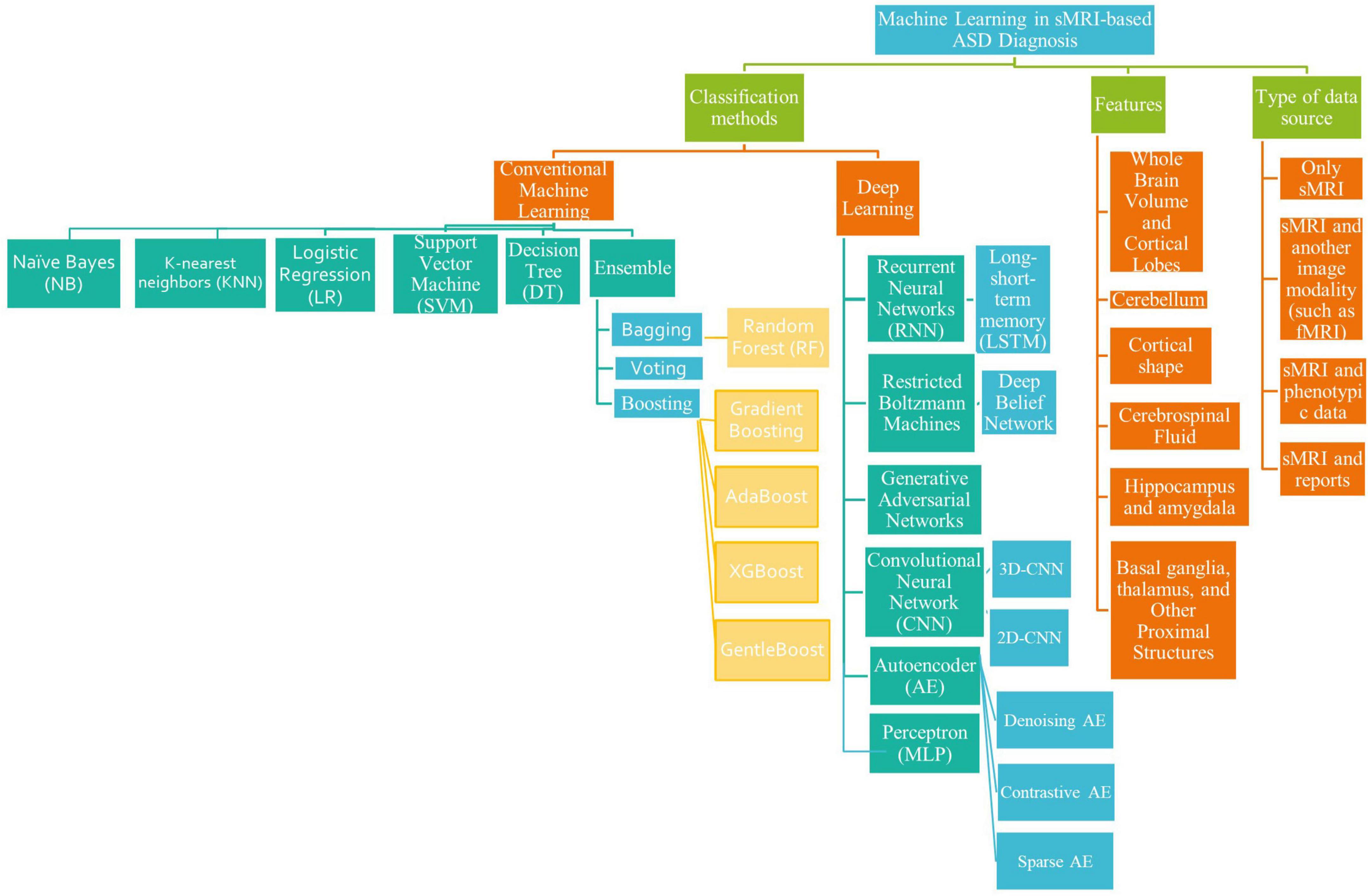
The survey taxonomy describes the methods, scan techniques, and features that are based on brain classification for ASD diagnosis (see Figure 1). This study looks at the age and number of subjects, features/biomarkers, types of scan modalities, datasets used, preprocessing tools, classification algorithms, and evaluation measures.

FIGURE 1

Figure 1. A literature-based taxonomy for ML-based ASD classification.

After the introduction, there are six sections in this article. Section 2 discusses the sMRI features and methods of extracting them. In Section 3, the general pipeline for ML and algorithms common in ASD research is described. In Section 4, ML/DL’s recent applications for diagnosing ASD using sMRI are presented, along with a description of the most consistent discriminatory biomarkers for diagnosing ASD across studies. Before concluding, we will evaluate the present research’s limits and discuss future directions that we believe will help researchers decide which studies to conduct. The review also provides a tabular summary of all articles, allowing readers to evaluate the area swiftly.

In summary, the purpose of this review is (a) to demonstrate ML/DL progress in brain ASD classification and (b) to identify open research challenges for developing effective ML/DL classification methods for the autistic brain.

Structural magnetic reasoning imaging and features extraction

Including MRI, all medical imaging techniques are diagnostic in themselves. It generates non-invasive visual representations of the body’s interior that are utilized to extract insights for clinical evaluations and describe pathological processes (Zhang L. et al., 2020).

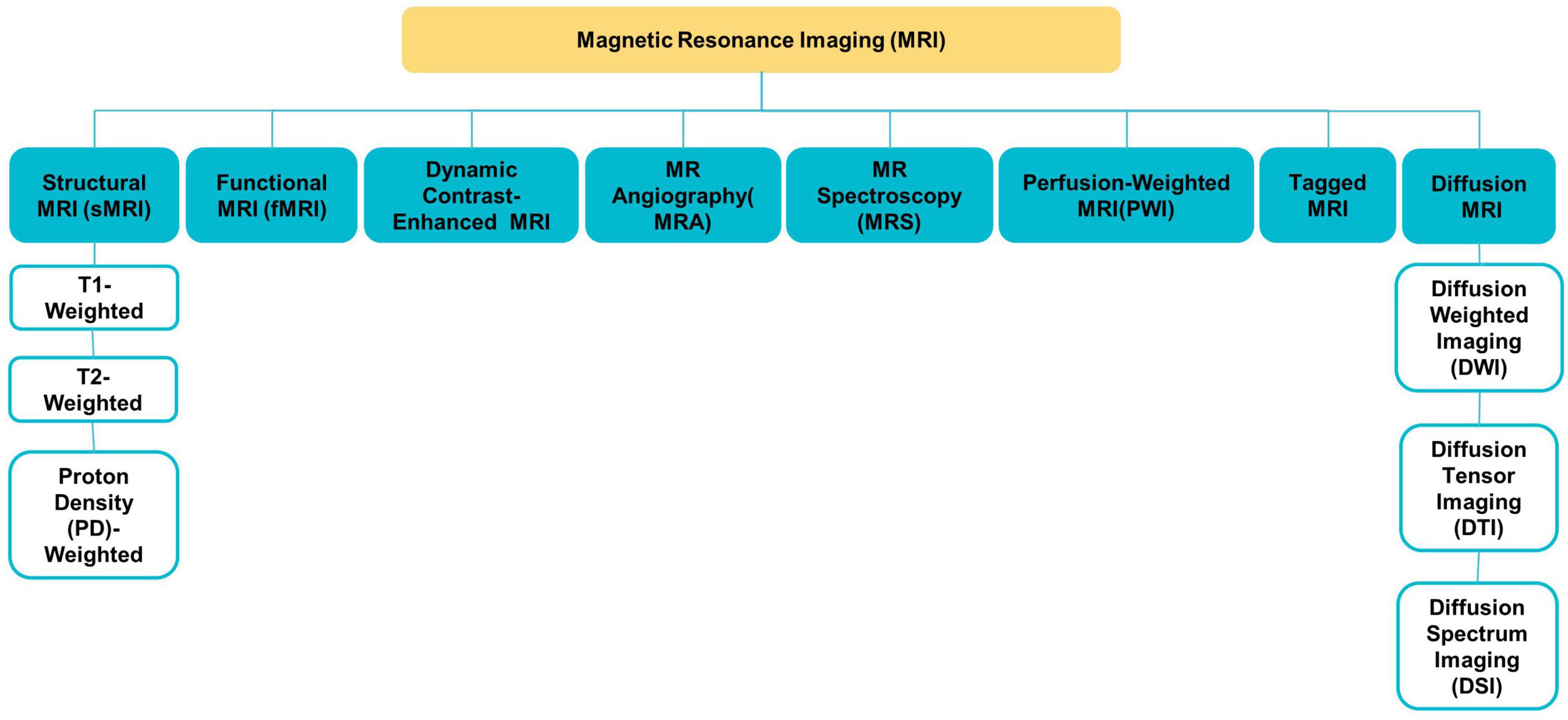
Various MRI modalities, such as sMRI, fMRI, and diffusion tensor imaging (DTI) (see Figure 2), have been employed in studies to capture the effect of ASD on the brain from a range of perspectives (Ahmad et al., 2014).

FIGURE 2

Figure 2. Different MRI modalities.

sMRI is commonly used to examine brain morphology because of its high contrast sensitivity, spatial resolution, and the fact that it does not need exposure to ionizing radiation; this is especially significant for children and adolescents (Ali et al., 2022). sMRI delivers various sequences of brain tissue (e.g., T1, T2, and FLAIR) created by altering excitation and repetition durations to view multiple brain regions (Eslami et al., 2021).

With the explosion in data in medical imaging of various types, medical image analysis and the extraction of clinically relevant information have become a major challenge. AI technologies are needed to enhance health care outcomes by boosting sophisticated analytical skills. Medical imaging research on CAD is expanding quickly. Because items such as organs may not be represented accurately by a simple equation; thus, medical pattern recognition requires “learning from examples” (Suzuki, 2013). One of the most popular uses of ML is the classification of objects such as brains into certain classes (e.g., healthy or autistic) based on input features (e.g., GM volume).

In CAD systems, the sMRI image undergoes steps like acquisition, image enhancement, feature extraction, the region of interest (ROI) definition, result interpretation, etc. Feature extraction conducts scientific, mathematical, and statistical operations or algorithms to discover quantifiable features/biomarkers from an sMRI image which can be used as inputs to ML models to detect brain disorders. Morphometric features and morphological networks are the two main types of features that can be extracted from sMRI.

This section discusses the most used methods for defining features from sMRI data.

Morphometric features

Morphometric features include two main types, geometric and volumetric features, which can be employed for the MRI-based diagnosis of ASD. Geometric features are two-dimensional surface features associated with the cerebral cortex, such as curvature, surface area, and thickness (Ali et al., 2022). While volumetric features usually refer to the size of the subcortical structures [e.g., white matter (WM) volume] (Ecker et al., 2010). Some tools, such as FreeSurfer, and Statistical Parametric Mapping (SPM), can easily extract morphometric features (Shen et al., 2017).

Morphological networks

This method connects morphological data from various brain regions (Eslami et al., 2021).

Depending on the spatial scale, features can be produced in one of three ways: voxel-based, region-based, or network-based (Xu et al., 2021).

Researchers can use pre-defined regions and extract data specifically from voxels within those regions to find specific findings in brain scans. This is called an ROI-based analysis (Chen et al., 2011). Experts manually or semi-manually identify brain regions, which takes a long time. This type of research is also limited by the number of brain regions that can be examined. By increasing the number of voxels in a target ROI, the statistical power increases (Chen et al., 2011). ROI detection algorithms fall into four categories: (1) based on changes in voxel values, like edge detection algorithms; (2) based on human-computer interaction. (3) those that use human visual characteristics, such as color detection algorithms; (4) DL-dependent, like Recurrent Attention Model (RAM) and Class Activation Mapping (CAM) (Ke and Yang, 2020).

In contrast, voxel-based approaches can detect statistically significant tissue density differences between the two groups (Seyedi et al., 2020). It is more appropriate given the lack of consensus on which brain areas are important in ASD (Eslami et al., 2021). Voxel-wise techniques include voxel-based morphometry (VBM), surface-based morphometry (SBM), and tensor-based morphometry (TBM) (Chen et al., 2011; Chen T. et al., 2020). VBM’s main characteristics are the density and volume of GM, WM, and cerebrospinal fluid (CSF) (Chen et al., 2011). TBM, unlike VBM, does not compute volume information for various tissue types separately (Chen T. et al., 2020). On the other hand, SBM research focuses on cortical topographic measurements like thickness, curvature, and area (Chen et al., 2011). The SBM method excludes ASD-linked subcortical regions like the basal ganglia (Chen T. et al., 2020). Neurological disease can damage multiple brain regions, making voxel-based or region-based approaches ineffective (Islam, 2019). Network-based methods are used to extract global features like voxel or ROI interaction patterns (Eslami et al., 2021).

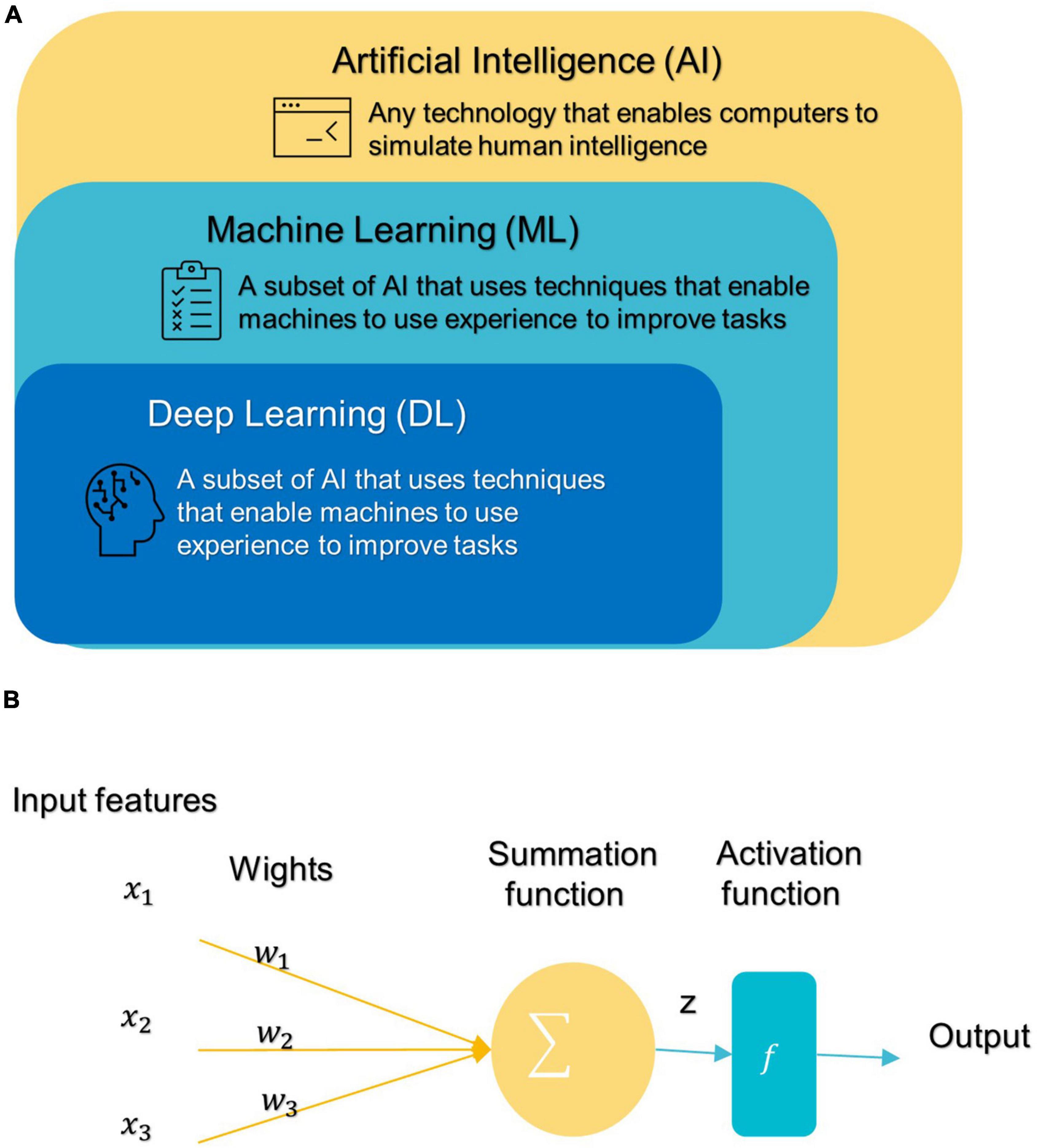
General machine learning pipeline and common algorithms for classification of autism spectrum disorder

In 1959, Samuel coined the term “machine learning” (ML), which is a subfield of artificial intelligence (AI) that allows machines to learn from data without being explicitly programmed (see Figure 3A; Samuel, 2000; El Naqa and Murphy, 2022). ML has three broad categories: supervised, unsupervised, and semi-supervised learning algorithms (Eslami et al., 2021). Deep learning (DL) is a subset of ML that is based on artificial neural networks inspired by the way human neurons communicate (Eslami et al., 2021).

FIGURE 3

Figure 3. (A) Branches of Artificial Intelligence Science. (B) An artificial neuron’s architecture. Each input × is associated with a weight w. The sum of all weighted inputs is passed onto an activation function f that leads to an output.

Most conventional ML algorithms required human intervention to extrapolate specific data features and patterns before consuming them to learn from Eslami et al. (2021). Handcrafted feature extraction is an expensive procedure (Nogay and Adeli, 2020). DL can automatically detect and extract representations (features) with strong discriminatory power from input data (Liu et al., 2020).

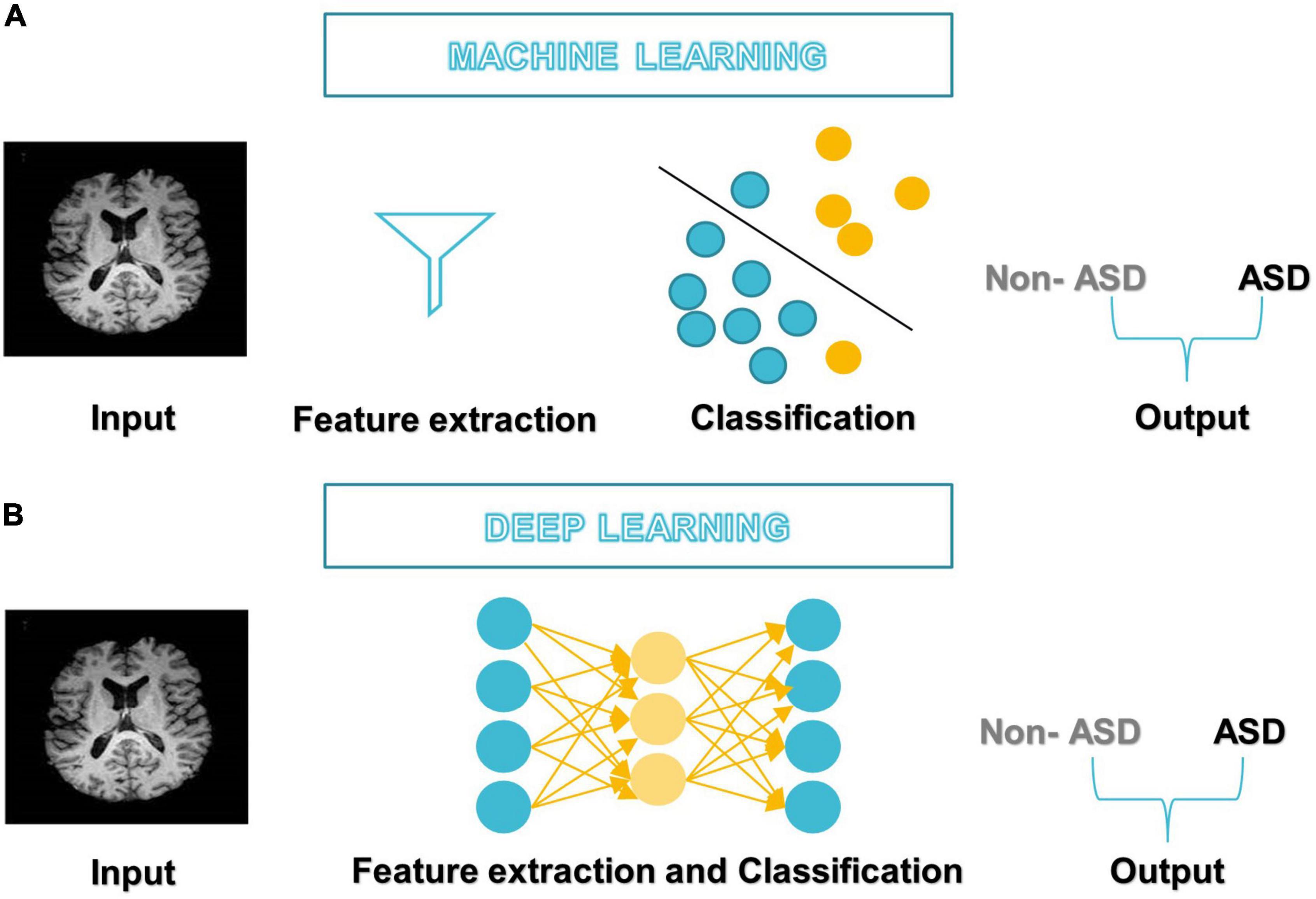
After DL’s success in the ImageNet challenge in 2012, it only took 5 years for the first DL algorithm for medical imaging (Krizhevsky et al., 2012). A deep neural network (DNN) (Misman et al., 2019) has one or more hidden layers between the input and output layers. Each layer is made up of layers of nodes known as artificial neurons (see Figure 3B). Each layer’s representation is transformed into the most abstract and composite layer. The purpose of hidden layers is to automatically collect valuable features from input and apply them in the classification stage (Liu et al., 2020). Figure 4 represents the difference between ML and DL.

FIGURE 4

Figure 4. Differences between (A) ML-based studies workflow and (B) DL-based studies workflow.

Therefore, the application of ML models that also include DL to diagnose disorders has increased rapidly in recent years. So, in the next section, we focus on describing ML models and the general framework for their application in ASD diagnostic studies to make them accessible to neuroscientists.

A general machine learning based framework for classification of autism spectrum disorder

Figure 5 illustrates a generic pipeline for establishing an ML-based ASD diagnosis. ASD classification may be broken down into four components: (a) data collection and preprocessing; (b) feature extraction and selection/reduction; (c) model training; and (d) model testing and performance evaluation.

FIGURE 5

Data acquisition and preprocessing

The first step in building a good classification framework is always to obtain the right data that represents the entire field of interest, is suitable for the learning objective, and is consistent, complete, and adequate.

Preprocessing is then mainly used to enhance the visual impression of an image. Due to the complex structure of neuroimaging data, failure to preprocess them might have a negative impact on the final diagnosis (Wujek et al., 2016; Khodatars et al., 2021). There are two layers to the preprocessing of neuroimaging data: low-level processing and high-level processing. Low-level processing steps such as brain extraction, normalization, spatial smoothing, and atlas registration [e.g., automated anatomical labeling (AAL), Harvard Oxford Atlas (HO)] are frequently repeated across studies and are typically performed with pre-built toolboxes [e.g., FreeSurfer (Fischl, 2012), FSL (Jenkinson et al., 2012), iBET (Dai et al., 2013), and SPM (Khodatars et al., 2021) to minimize processing time and improve a study’s reproducibility (Khodatars et al., 2021)]. High-level processing [e.g., data augmentation (DA) (Eslami et al., 2019), and sliding window (Li X. et al., 2018)] is applied to the data following typical preprocessing methods to increase the accuracy of ASD detection. It is difficult to implement and repeat complex processing steps in neuroimaging, so pipelines such as Nipype or LONI have been found that combine the power of analytical tools with the speed of data processing as well as facilitate the repetition of the same steps between different studies (Khodatars et al., 2021).

Feature extraction, selection/reduction

A feature is any measurable property extracted from the source dataset regarding the class. Through features engineering, neuroimaging data is transformed into trustworthy and biologically relevant features that greatly influence data separation (Xu et al., 2021). The “dimensionality curse” problem is quite common in medical imaging analysis because the sample density decreases exponentially as the number of features increases. Some of these features may be redundant or irrelevant to the prediction; removing them does not result in a significant loss of information (Xu et al., 2021). If there are too many features compared to the number of samples, then more training samples will be required; otherwise, there is a risk of model “overfitting,” which causes the model to perform well on training data but badly on unseen or new data; such models are deemed non-generalizable (Kim and Na, 2018).

The most efficient technique for avoiding the curse of dimensionality is feature selection/reduction, which reduces noise and redundant features and facilitates the understanding of neural mechanisms of diseases by preserving the most discriminant features while increasing model accuracy and generalizability (Kim and Na, 2018). There are two basic ways to feature selection: supervised and unsupervised. Supervised approaches need the training label to choose informative and discriminative feature dimensions and exclude others (e.g., exclude irrelevant variables) (Saeys et al., 2007). This strategy has three subtypes: filter, wrapper, and embedding (Xu et al., 2021). In contrast, unsupervised approaches, such as principal component analysis (PCA) build low-dimensional feature representations by combining the original features in linear or non-linear ways without requiring the training label (Kim and Na, 2018; Xu et al., 2021).

Model training

The model and a suitable training method are chosen depending on the learning goal and data requirement. The hyperparameters that determine the model’s architecture (e.g., number of neurons, activation function, batch size, etc.) are then optimized for optimum performance, model generalization, and loss function reduction (Kim and Na, 2018; Xu et al., 2021). Hyperparameter tuning/optimization is the process of determining the optimal combination of hyperparameter values to get maximum data performance in an acceptable amount of time (Rojas-Domínguez et al., 2017). Hyperparameters differ amongst models and must be established before entering the training phase since they do not change and are not learned during training. Unfortunately, there is no mechanism to determine “what is the best approach to setting the model’s hyperparameters to minimize loss?” Thus, research and experiment are used to find the optimal option. In general, this process entails the following steps: defining a model, determining the range of possible values for all hyperparameters, sampling hyperparameter values by any of the different techniques to search for the ideal model structure, such as GridSearchCV and RandomizedCV, determining prediction error and other evaluation criteria to evaluate the model (Ali et al., 2021; Eslami et al., 2021). The prediction error is computed by applying the loss function to the expected value and the underlying truth. The choice of loss functions depends on the nature of the problem and the desired outcome. Mean squared error and mean absolute error are widely used in regression problems, while cross-entropy loss is utilized for classification (Eslami et al., 2021).

Model testing and performance evaluation

The model usually performs well in the training phase, but generalization requires further investigation in the testing phase. Test data should not be used during the training phase to avoid bias. Since most clinical data contains small samples that may lead to an insufficient model for training, unbiased cross-validation (CV) is frequently used to validate the model’s effectiveness and assess the data’s predictive capability. K-fold CV is a common validation method. To use it, the data set is divided into K subsets (also called folds) and used k times. The training process is initially performed on the K-1 subset, saving the remaining subset for later use as a test set and ensuring that the test and training sets do not overlap throughout each iteration (Xu et al., 2021).

Common confusion matrix-based quantitative measures of model performance are accuracy (ACC), sensitivity (Sen), specificity (Spe), positive predictive value (PPV), and negative predictive value (NPV). Whereas positive samples are autistic individuals and negative samples are healthy controls (HCs), true positive (TP), and true negative (TN) rates refer to the number of correctly classified positive and negative instances, respectively, while false positive (FP) and false negative (FN) rates refer to the number of incorrectly classified positive and negative instances, respectively (Uddin et al., 2017; Mostapha, 2020).

In statistics, accuracy is the proximity of repeated measurement results to the true value. It is also known as “diagnostic effectiveness” (Kong et al., 2019). The proportion of ASD disorders that were correctly diagnosed is referred to as sensitivity. “Specificity” is the proportion of typical developmental people whose ASD disorder was precisely excluded (Mostapha, 2020). The PPV of a test answers the question: “How likely is it that a patient who provided a positive test result has ASD?” While the NPV of a test provides an answer to the question: “How likely is it that a patient who gives a negative test result will not have ASD?”

Each metric describes a different aspect of the model’s power (Xiao et al., 2017). The receiver operating characteristic (ROC) curve is also widely used (Xu et al., 2021). This graph depicts the true positive rate (Sen) vs. false positive rate (1-Spe). The ROC curve is used to establish the appropriate cut-off point for both specificity and sensitivity. All possible combinations of Spe and Sen achievable by varying the test cut-off value can be summed up by utilizing the area under the receiver operating characteristic curve (AUC) parameter. AUC, or the area under the ROC curve, can never be more than 1, and the bigger it is, the more accurate the test is (Li H. et al., 2018). The F1 score is calculated by averaging the PPV and Sen scores. Therefore, this score takes both FP and FN into account (Panja et al., 2018; Wang et al., 2021).

ACC=T⁢PT⁢P+T⁢N+F⁢P+F⁢N×100(1)

Sen=T⁢PT⁢P+F⁢N×100(2)

Spe=T⁢NT⁢N+F⁢P×100(3)

PPV=T⁢PT⁢P+F⁢P×100(4)

PPN=T⁢NT⁢N+F⁢N×100(5)

F1-score=2*T⁢P2*T⁢P+F⁢P+F⁢N×100(6)

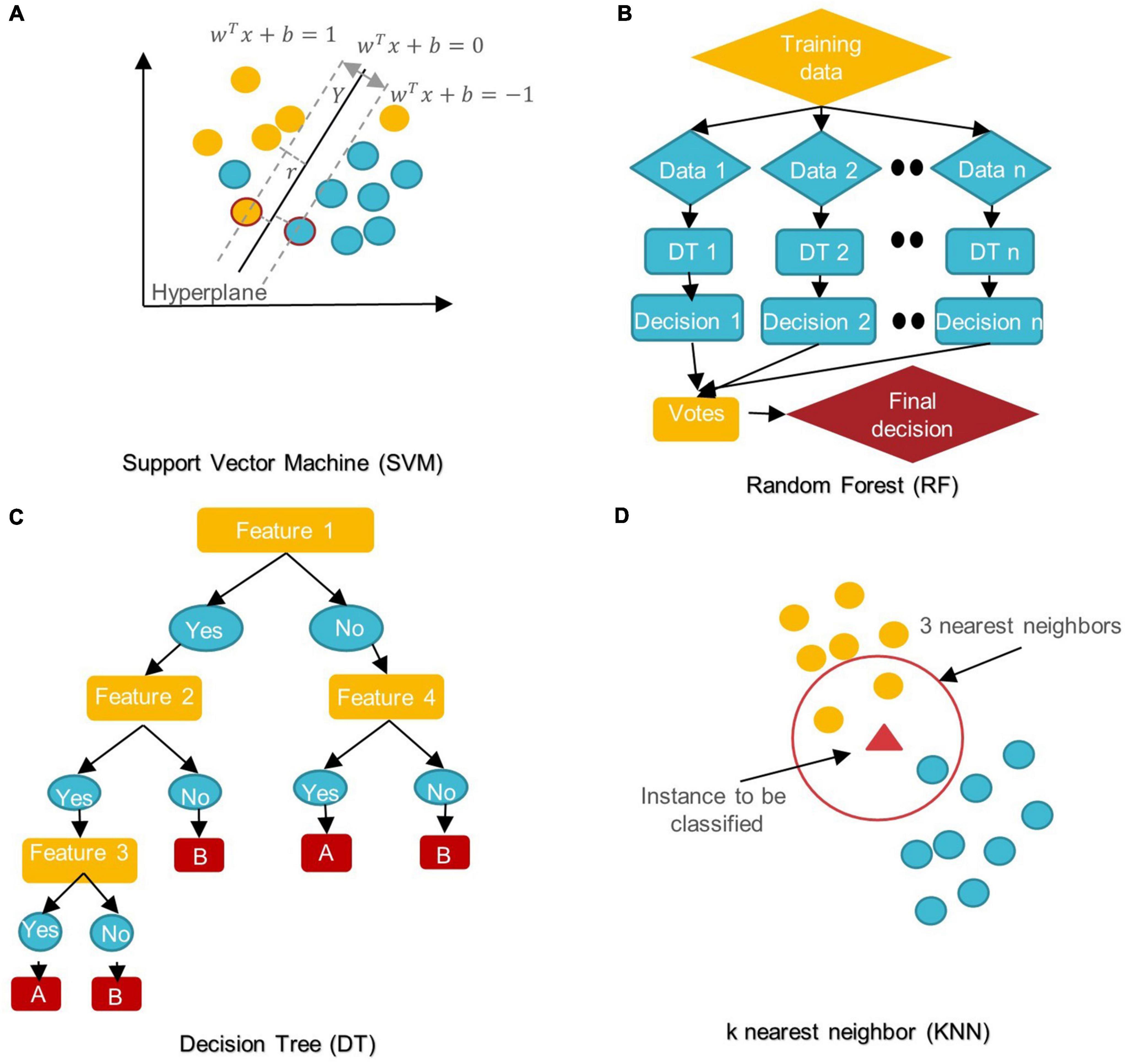
Common conventional machine learning and deep learning algorithms in autism spectrum disorder diagnostic research

In the last 5 years, several ML/DL models have been used in ASD research. Support Vector Machine (SVM), Random Forest (RF), Decision Tree (DT), Logistic Regression (LR), Naïve Bayes (NB), Boosting, and k-Nearest Neighbors (KNN) were among the most popular conventional ML algorithms (see Figure 6).

FIGURE 6

Figure 6. Schemes of conventional ML algorithms commonly used in MRI-based studies to diagnose ASD (A) SVM: support vector machine; (B) RF: random forest; (C) DT: decision tree; (D) KNN: k nearest neighbor.

SVM aims to find the best decision boundary that increases the margin between classes in a high-dimensional space (Cortes and Vapnik, 1995). In SVM’s final discrimination function, only the data points (support vectors) closest to the hyperplane control the movement of the hyperplane that splits the data (Xiao et al., 2017). The kernel tricks of SVM can handle nonlinear classification, but they make the model harder to interpret (Panja et al., 2018). SVM is not influenced by outliers and is not sensitive to overfitting, but it is not optimal for a large number of features (Cortes and Vapnik, 1995; Xiao et al., 2017).

DT is a rooted directed tree with a flowchart-like structure that depicts the different consequences of a set of decisions. A DT contains branches that represent the data set’s features and leaf nodes that represent the outcome or decision (Liu et al., 2020). DT has good interpretability as it can approximate complex decision areas through a set of straightforward decision-making rules (Xu et al., 2021).

RF is made up of DT ensembles. RF uses random sampling with replacement (bootstrapping) to create many DTs during training. The forest is determined by the majority vote of the trees; hence, RF may give more accurate predictions than learning with a single DT (Uddin et al., 2017; Yin et al., 2020).

LR is a probabilistic method for estimating the statistical importance of features. Its purpose is to determine the values of the parameters that reflect all input variables. LR employs a logistic function in its most basic form to represent a binary dependent variable. It may also be modified to simulate many event classes (Uddin et al., 2017; Liu et al., 2020).

NB classifiers are based on Bayes’ theorem with high predictor independence. The NB classifier assumes that the effect of a predictor (x) on a particular category (c) is independent of the other predictors’ values. Despite its simplicity, NB classifiers often outperform more complex classification methods, especially for large data sets (Xiao et al., 2017; Bilgen et al., 2020; Chen T. et al., 2020).

In KNN, the data is categorized into several specified groups. It is carried out in such a way that all data points within the group are classified as homogeneous or heterogeneous when compared to data from other groups (Dekhil et al., 2021).

The boosting algorithm is an ensemble algorithm that transforms weak learners into strong ones. Weak learners have a weak connection to correct categorization. A strong learner is closely related to true classification (Bilgen et al., 2020).

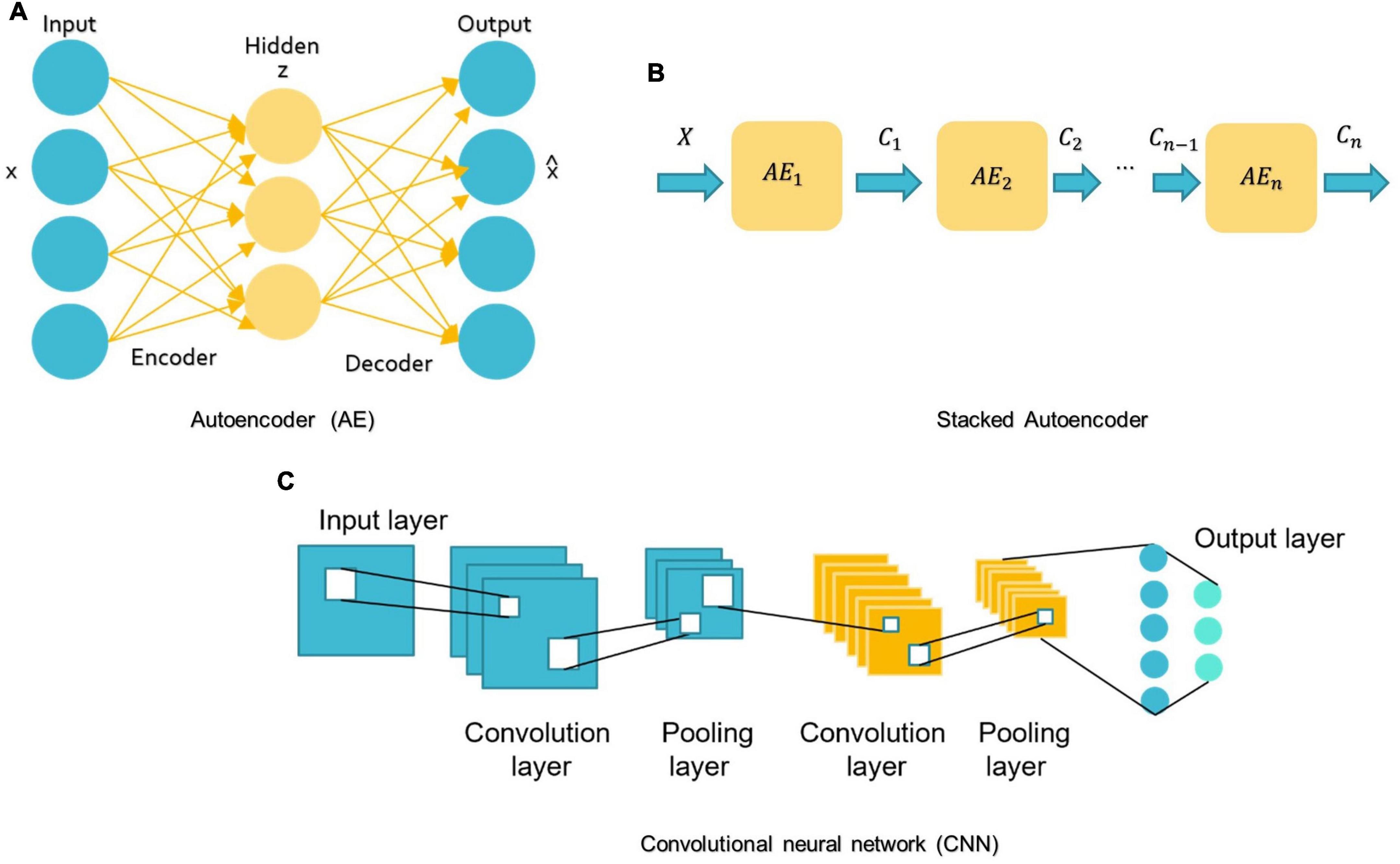
For DL, there are several models such as Convolutional Neural Networks (CNN), deep generative models [e.g., Autoencoders (AE), Deep Belief Networks (DBN), and Generative Adversarial Networks], Multi-layer Perceptron (MLP), Recurrent Neural Networks (RNN), and Graph Convolutional Networks (GCN) that have been employed in various areas like computer vision, natural language processing, and speech recognition (Zhang L. et al., 2020; Khodatars et al., 2021). The first four were mostly used in reviewed ASD studies (see Figure 7).

FIGURE 7

Figure 7. Schemes of DL algorithms are commonly used in MRI-based studies to diagnose ASD. (A) AE: autoencoder; (B) Stacked Autoencoder; (C) CNN: convolutional neural network.

MLP belongs to the class of feedforward neural networks with the same number of input and output layers but may have multiple hidden layers. MLP forward data from one layer to the next after linear and non-linear transformations (Libero et al., 2015; Mellema et al., 2019).

A basic AE requires two networks: an encoder network E and a decoder network D (see Figure 7A; Mostapha, 2020). The first network encodes the input data x into the low-dimensional space z, which is then used to decode and reconstruct the x data (Mostapha, 2020). Various types of AE, including contractive, sparse, and denoising AEs, were used in research for dimension reduction and to investigate the highly discriminative representations from neuroimaging data, but the spatial structure of data is often discarded (Kong et al., 2019). Stacking AEs, such as the stacked sparse AE (SSAE) is possible (see Figure 7B). Stacked AEs can learn faster than a single autoencoder (Zhang L. et al., 2020).

On the other hand, CNN can leverage the spatial information of sMRI data and deal with complex image processing problems. A standard CNN has multiple layers that process and extract features from data, as shown in Figure 7C. A CNN has many convolutional layers with multiple filters to perform the convolution operation. A filter (also called a kernel) determines the presence of certain features or patterns in the input. Next comes the Rectified Linear Unit to perform operations on the elements and produce a feature map (or activation map). The feature map is then fed to a pooling layer. Pooling is a down-sampling process that reduces the dimensions of a feature map. This makes the learning process relatively less expensive. Max and average pooling are the most widely used pooling techniques. The pooling layer flattens the 2D arrays of the pooled feature vector to create a single long vector by flattening it. The fully connected layer comes last, and it contains some hidden neural network layers. This layer classifies the image into different categories (LeCun et al., 2010; Ozonoff et al., 2011).

In the context of sequential data, RNNs are particularly beneficial since each neuron may retain the result of the previous stage in its internal memory and pass it to the current stage as input (Dua et al., 2020). This means RNNs can capture long-term relationships between input symbols (Mittal and Umesh, 2021). But training these RNNs is very costly (Dua et al., 2020). Moreover, early RNNs had simple recurring layers but they had a vanishing gradient problem and didn’t work for long data sequences (Dua et al., 2020). Long-short-term memory (LSTM) is the most prevalent architecture of RNNs used to solve these problems (Eslami et al., 2021; Quaak et al., 2021).

Highlighted research

Recent advances in neuroscience and brain imaging and their combination with ML techniques using the methods described above allow us to understand the brain and the different regions implicated in ASD and their interaction. In this section, first, we summarize recent research on possible sMRI-based ASD biomarkers. Part 2 includes studies that only used conventional ML algorithms. Then we look at studies that benefited from DL algorithms.

Identification of the potential autism spectrum disorder biomarker from structural magnetic resonance imaging Whole brain volume and cortical lobes

Although the etiology of ASD remains unclear, for decades, an abnormally rapid increase in head circumference has been observed in some children with autism (Kanner, 1943; Pagnozzi et al., 2018). In light of the substantial correlation between head circumference and total brain volume (TVB), various volumetric studies have studied brain volume as a quantitative measure retrieved from sMRI (Pagnozzi et al., 2018). Atypical brain development in infancy may be used as an early ASD biomarker. Based on research by Hazlett et al. (2012), ASD children aged 2–4 had a larger brain than their peers, and in the next study (Hazlett et al., 2017), showed that ASD’s high-risk family members (HR) (Those who had a sibling with autism) at 6–12 months of age showed significantly higher cortical surface area (SA) growth compared to HCs, followed by an enlargement of TVB at 24 months of age as correlated with the severity of social autism. The SA growth rate increased mainly in the left and right middle occipital gyri, right lingual gyrus area, and right cuneus (Hazlett et al., 2017). Differences in the right occipital lobe are consistent with other studies (Irimia et al., 2018; Landhuis, 2020) that explain visual perception differences between ASD patients and HCs. This appears to correlate with a report by Irimia et al. (2018) that discovered the ASD group had higher areas and connectivity densities in the cuneus, occipital lobes, and the superior and transverse occipital sulci than the HC group. The ventral frontal lobe of ASD patients and HCs differs significantly (Irimia et al., 2018). The superior temporal gyrus curvature appeared smaller in ASD males than in ASD females, consistent with other results on ASD sex differences and their memory processing ability (Xiao et al., 2017) findings. Some studies link ASD to biological sexual differentiation, which might also explain the disparity in reported brain volume anomalies (Hazlett et al., 2012; Irimia et al., 2018). Adult autistic brain GM/WM volumes increased differentially and decreased across distinct areas, in contrast to early childhood increases in global volume measures (Akhavan Aghdam et al., 2018; Gorriz et al., 2019). This may be due to autism’s heterogeneity and potential subtle structural impacts or VBM’s limits, as VBM is sensitive to many artifacts, such as brain structure misalignment, which may mislead statistical analysis (Pagnozzi et al., 2018). In Dekhil et al. (2020) reported that changes in the size and shape of the cerebral cortex leading to an altered arrangement of WM fibers and changes in GM/WM; this, on its part, is relevant to identifying circuit abnormalities associated with autism. In Akhavan Aghdam et al. (2018), some differences exist in GM volume, particularly in the frontal and temporal regions, hippocampus, caudate nucleus, or other parts of the basal ganglia, amygdala, as well as the cerebellum. These areas include most of the TVB. TVB or intracranial volume (ICV) are essential factors for volumetric analyses of the brain (Kijonka et al., 2020). TVB = GM + WM (Hazlett et al., 2017). ICV is the sum of TVB and CSF volumes (Gorriz et al., 2019).

Cortical shape

Cortical thickness (CT), SA, the gyrification index (GI), and the sulcal morphology of the cerebral cortexes are all ROIs when investing in volume changes connected to ASD (Pagnozzi et al., 2018). The observed differences among studies are accentuated by the lack of agreement in designating ROIs. The CT is the shortest distance between the GM/WM border and the pial surfaces (Xiao et al., 2017). SA is the surface area of the WM. To find the cortical volume, multiply the SA by the CT (Xiao et al., 2017). CT levels in various brain regions have risen or fallen in different studies (Grimm et al., 2015; Raamana and Strother, 2020).

Motivated by evidence that regional CT measures can indicate cortical maturation and cortical-cortical connectivity and that ASD is characterized by delayed development, some studies (Moradi et al., 2017; Zheng et al., 2019) have supported CT scores as an ASD biomarker. For example, in Moradi et al. (2017) authors demonstrated a positive association between Autism Diagnostic Observation Schedule (ADOS) test-derived symptom severity and CT measurements. They also noted that age could affect CT and that the severity of the disorder determines age-related change. Their results also revealed a greater importance of the right hemisphere for predicting ASD severity than the left hemisphere. In Itani and Thanou (2021), the CT was higher in ASD than HCs in all ROIs identified at work. A statistically significant difference is shown in the superior frontal gyri, bilateral middle temporal gyri, right pars orbitalis, right insula, entorhinal cortex, and left superior temporal gyrus. Irimia et al. (2018) revealed similar findings in CT of the temporal lobes and superior temporal gyri. In contrast, Xiao et al. (2017) indicate that the left hemisphere is superior in distinguishing ASD. The left caudal anterior cingulate, the left parahippocampal, the left pars triangularis, and the left precuneus all have the same predictive value for ASD patients in the left hemisphere. According to Xiao et al. (2017), with neuroimaging data, the thickness-based classification of ASD performs better than both volume-based and SA-based classification. Broca’s area contains a part of the inferior frontal gyrus known as the Pars triangularis that contributes to language and social interaction difficulties. The caudal anterior cingulate is part of the social brain and mirror system hypothesis and cognitive regulation of behavior, including working memory, attention management, and decision making. The parahippocampal gyrus is critical for memory encoding and retrieval (Xiao et al., 2017). Thinning of the cerebral cortex within this region may affect the neural basis for risk disregard in autistic people (Xiao et al., 2017). Self-relevant mental images are identified in the anterior part of the precuneus, with posterior regions implicated in episodic memory visuospatial imagery, episodic memory retrieval, and self-processing operations. In summary, disruption in those four areas may be connected to ASD social issues and repetitive behaviors.

Cerebrospinal fluid

CSF is a fluid that surrounds the entire surface of the brain and the spinal cord and flows between the brain membranes. Although CSF is not technically a part of the human brain, it circulates nutrition, removes waste items generated by cerebral metabolism, and protects the brain from harm. However, CSF volume may be an indirect indicator of tissue loss in brain regions (Pagnozzi et al., 2018) and thus may be an important biomarker of ASD-induced brain-related changes. In young autistic children, an abnormal elevation of CSF can also occur, including movement, communication, and ASD status (Shen et al., 2017; Mostapha, 2020).

Cerebellum

The prefrontal cortex and cerebellum (Gao et al., 2022; Wang et al., 2021) and the temporal cortex (Wang et al., 2021) help classify structural covariance brain networks. Basic conscious motions are physically and functionally linked to the prefrontal cortex, and its abnormality is associated with ASD’s emotional and social domain. Studies have indicated that the superior temporal gyrus and the medial temporal cortex have direct connections that promote the memory for sound detection.

In addition, the cerebellum is essential for cognitive functions, memory, emotion, and language (Gao et al., 2022). The ASD and HC groups differed significantly in the choroid plexus, cuneus, left putamen, and cerebellar cortex (Pinaya et al., 2019).

Hippocampus and amygdala

The medial temporal lobe houses the hippocampus and amygdala, two interconnected subcortical structures. The hippocampus helps develop associative, spatial, episodic, and declarative memory. Similarly, the amygdala is involved in emotion and fear control and the recognition of facial expressions (Pagnozzi et al., 2018).

The amygdala and hippocampus have been linked with ASD-related deficits, including social cognition, eye-gaze direction perception, and emotion (Li et al., 2019b).

Researchers found that the ASD group had significantly less parahippocampal volume than the HC group (Irimia et al., 2018). As for the interaction with sex, autistic females had a larger right parahippocampal gyrus volume than autistic males.

Utilizing ML, another study found that the hippocampus plays a role in ASD (Fu et al., 2021). By comparing their findings with previous work on Alzheimer’s disease, they conclude that the overall severity of ASD-related morphological changes in the hippocampus is less pronounced or that the abnormality is more distributed in hippocampus areas.

In Li et al. (2019b), ASD was associated with significant enlargement of the amygdala and CA1-3 of hippocampal volumes in the right and left hemispheres. CA1-3 expansion could represent upregulation, reinforcing fear of communicating with the environment or others.

Basal ganglia, thalamus, and other proximal structures

The basal ganglia (BG) are neurons, also called nuclei, located in the depths of the cerebral hemispheres of the brain. In addition to coordinating postural muscle movements, the BG is involved in many regular behaviors and routines, such as the grinding of teeth, eye movements, and emotion. Although few studies have examined the role of BG in ASD symptoms, structural and strategic evidence suggests that ASD is linked to subcortical regions, including BG (Sivapalan and Aitchison, 2014; Pagnozzi et al., 2018; Ke et al., 2020). According to Irimia et al. (2018), those with ASD exhibited larger areas and volumes in some limbic structures such as the cingulate gyrus and the pericallosal sulcus. The temporal lobe, corpus callosum, middle cerebellar peduncle, caudate, and cingulate nucleus were the most relevant regions identified for predicting ASD in Guo et al. (2021).

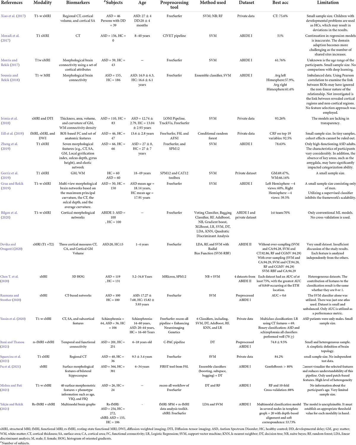
Conventional machine learning-based autism spectrum disorder classification applications

Several researchers have developed ML algorithms employing sMRI (Moradi et al., 2017) or multimodal data (Eill et al., 2019) to diagnose ASD or uncover novel biomarkers for it (Table 2, summarizing all ML-based studies). SVM has been extensively evaluated, with ACCs ranging from 45 to 94% on various ASD datasets (Morris and Rekik, 2017; Squarcina et al., 2021). In addition, various additional conventional ML models, such as NB (Xiao et al., 2017), KNN (Yassin et al., 2020), AdaBoost (Bilgen et al., 2020), and RF (Devika and Oruganti, 2020), have been examined. With an ACC = 94.29%, SVM was the most accurate of the ASD classification models, despite having the smallest data set (n = 35) (Devika and Oruganti, 2020). Zheng et al. (2019) use SVM and a multi-feature network to differentiate between ASD and HC. Their ACC is 78.63%.

TABLE 2

Table 2. Summary of 20 ML-based ASD classification studies.

Individual variations in ASD symptom severity require individualized therapy based on associations between brain structure and clinical assessments of ASD risk, such as the ADI-R (Xiao et al., 2017) and ADOS (Moradi et al., 2017; Dekhil et al., 2021). Despite their limited scope, these studies are still noteworthy. In one study, RF, NB, and SVM were applied to 46 participants with ASD and 39 participants with developmental delay (Xiao et al., 2017). This study employed many differentiating features to increase classification accuracy: CT, cortical volume, and SA. The RF model was the most accurate, derived from the CT of 20 significant brain regions. Moradi et al. (2017) estimated ASD symptoms using ABIDE data and ADOS severity scores generated from CT measures. The authors suggested a method for creating a common space within various datasets to reduce inter-site heterogeneity called “domain adaptation.” At 51%, this research had the lowest ACC rate across studies. Dekhil et al. (2021) created a personalized CAD system using sMRI, rs-fMRI, and ADOS. The system produces a report for each subject that highlights ASD-affected regions. RF utilizing only rs-fMRI data produced 75% ACC, sMRI data produced 79% ACC, and combining the two produced 81% ACC. In another work (Dekhil et al., 2020), only sMRI and fMRI features were used to research brain region changes between ASD and HC groups to present a CAD system to help target therapeutic interventions. The system achieved good ACC (sMRI 0.75–1.00; fMRI 0.79–1.00) on a relatively large population using KNN and RF models.

Most research uses binary categorization. Some articles have many experiments. Gorriz et al. (2019), for example, divided participants into four groups based on gender and condition to compare ASD and HC brains. All binary categories “MH vs. FH,” “FH vs. FA,” and “MH vs. MA” (MH: male healthy, FH: female healthy, FA: female autism, MA: male autism) were developed to study gender differences in the diagnosis of ASD using SVM. Also, this article shows an example of different applications where binary classification applications of MH, FH, FA, and MA estimates were made twice; each time a distinct feature, either WM or GM volumes, was used to see which one could be most distinct in diagnosing ASD.

Like most previous research (Irimia et al., 2018), it suffers from the over-aggregation of features on insufficient sample size. Using MRI and DTI data, the study evaluated the applicability of SVMs for studying the relationships between an ASD diagnosis and gender. They demonstrated excellent ACC, but their findings cannot be generalized.

Network neuroscience is mostly focuses on fMRI-derived or DTI-derived FC features, which may neglect inter-regional morphological changes (Chen et al., 2011; Heinsfeld et al., 2018). Morphological brain networks (MBNs) may simulate this morphological connection between ROI pairs, in which the link between two regions encodes their morphological difference (Bilgen et al., 2020). The study (Morris and Rekik, 2017) employed SVM to evaluate the connectivity of cortical MBN collected just from sMRI. By concatenating low- and high-order network features, the authors extract features that are novel but lack biological value. Soussia and Rekik (2018) applied SVM and ensemble classifiers to complex MBNs, which represent shape-to-shape relationships between pairs of ROIs. Each network is associated with unique cortical features such as sulcus depth, curvature, and CT. But they didn’t apply any feature selection strategy. These studies also used specific ML approaches, leaving a large spectrum of methods unexplored for detecting ASD. To address this, a Kaggle competition was held to develop a suite of ML algorithms for diagnosing ASD utilizing MBN (Bilgen et al., 2020). The efforts of 20 teams were evaluated based on preprocessing, dimensionality reduction, and learning models. The two highest teams achieved ACCs of 70 and 63.8% using a powerful clustering algorithm called gradient boosting. Eill et al. (2019) also used a conditional RF ensemble algorithm and reported a high classification ACC of 92.5%.

Fu et al. (2021) postulate that prior studies on ASD classification using large datasets had low accuracy rates because they only considered SBM as scalar estimates (e.g., CT and SA) and neglected geometric information between features. Their application of the GentleBoost ensemble classifier to surface features of the bilateral hippocampus of male participants with ASDs and HCs. achieved an 80% ACC.

It has also been established that feeding an RF classifier with MRI and personal characteristics data improves ASD classification (Mishra and Pati, 2021).

Gao K. et al. (2021) developed a method for predicting the disease in 24-month-old infants utilizing sMRI and an XGBoost model. Some investigations used a histogram of oriented gradients (HOG) to analyze the gradient information of the aberrant region within the medical image (Ghiassian et al., 2016). Chen T. et al. (2020) found ASD biomarkers in children using a two-level morphometry classification framework based on the 3D HOG approach and NB model. Four ABIDE II locations achieved 0.75 AUC.

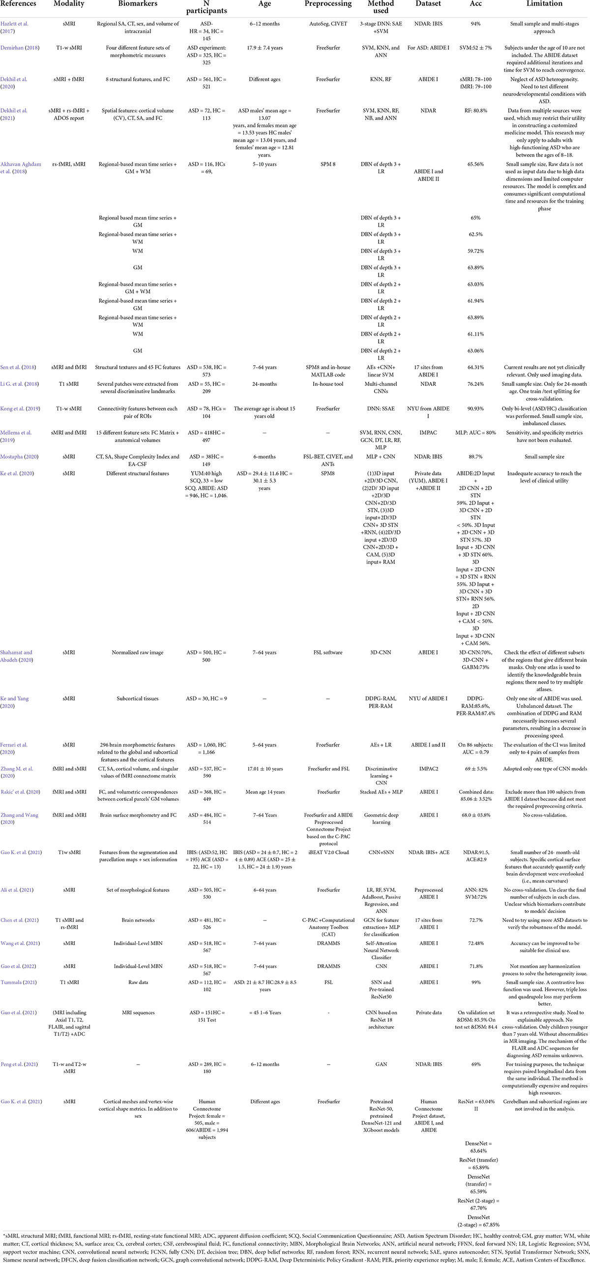
Deep learning-based autism spectrum disorder classification applications

Recently, DL approaches outperformed conventional ML methods and were hailed as a major AI accomplishment. Unlike conventional ML algorithms, DL can automatically extract hierarchical features from incoming data and intelligently categorize them inside the model (Mostapha, 2020). In medicine, DL frameworks have been used to classify ASD from sMRI data alone (Hazlett et al., 2017) or with other modalities (Dekhil et al., 2021; Table 3 a summary of studies on DL).

TABLE 3

Table 3. Summary of 25 DL-based ASD classification studies.

In Ali et al. (2021), a framework is presented that uses a recursive feature elimination method to select features and then trains linear, ensemble, and artificial neural network (ANN) models using them. ANNs enhanced categorization accuracy by up to 82%.

Several studies (Akhavan Aghdam et al., 2018; Sen et al., 2018; Mellema et al., 2019; Rakic’ et al., 2020) used sMRI and fMRI as inputs to the DL model. ASD disrupts FC between brain regions so many studies use FC neural patterns to distinguish ASD from controls. young autistic children were classified using the ABIDE I and II datasets and the DBN model (Akhavan Aghdam et al., 2018). The model achieved a maximum ACC (65.56%) combining three types of data (rs-fMRI + GM + WM).

Mellema et al. (2019) evaluated 12 classifiers using 915 IMPAC challenge dataset participants (Toro et al., 2018). These models comprise six non-linear shallow ML, three linear shallow, and three DL. For a fair comparison, the authors optimized each model’s hyperparameter using random search. To ensure that each model has the same training opportunity, random cross-validation was used. The dense feedforward network model achieves 80% AUC.

The reviewed studies employed various AE forms. In Sen et al. (2018), the authors utilized sMRI and rs-fMRI data to evaluate three ADHD and ASD learners. Learner 1 captures sMRI features using SAE-generated 3D texture-based filters and a CNN. Second learner computes non-stationary fMRI components. The final learner combines the structural and functional features of learners 1 and 2 and sends them to an SVM classifier, obtaining an ACC of 67.3% on ADHD data and 64.3% on ABIDE data, demonstrating that multimodal features can boost upset prediction accuracy.

Unlike fMRI, which is difficult to apply to infants, sMRI has gained interest for early ASD identification. sMRI is faster and contains infant-specific procedures, such as BCP (Howell et al., 2019; Gao K. et al., 2021). Deep generative algorithms were first utilized to predict ASD in infants using longitudinal data by Peng and others (Peng et al., 2021). Hazlett et al. (2017) developed a three-stage SAE model to diagnose infants with autism before the onset of behavioral signs. In contrast to most classification studies, which utilize cross-sectional data, a longitudinal dataset was used due to the relevance of a developmental approach to imaging, since ASD symptoms and implications may fluctuate over time (Lord et al., 2015). Despite the encouraging results in Hazlett et al. (2017), this multi-stage technique is inapplicable in clinical practice because it requires two scans at two different ages for tissue segmentation. An end-to-end and single scan-based method is used in Mostapha (2020). In Mostapha (2020), tissue segmentation was calculated automatically using a fully CNN.

MBNs that measure intracortical GM similarity are useful in the study of neurological disorders (Kong et al., 2019; Wang et al., 2021). The brain can be represented as a single view representation network or as a multi-view representation network (Graa and Rekik, 2019). Each view depicts a distinct morphological feature. Kong et al. (2019) used SSAE to learn low-dimensional brain connectivity patterns between each pair of ROIs from sMRI to build an individual brain network. Using only the 3,000 top F-scores features, the classifier had a 90.39% ACC. However, they used a small data set and did not depict potential biomarkers. The study (Gao et al., 2022) addressed this issue by identifying a biomarker using a Res-Net and gradient-weighted class activation mapping (Grad-CAM) on indiv