
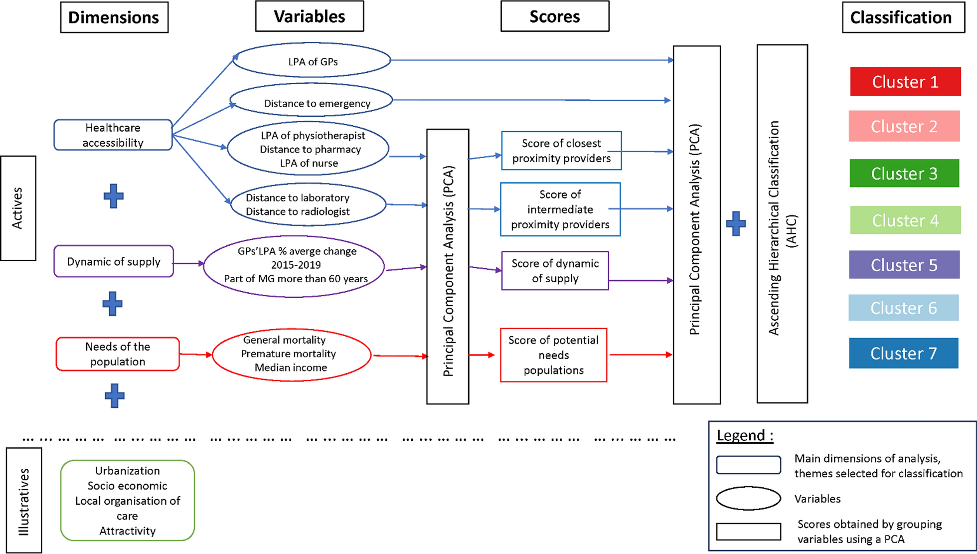
記住我


This section explains the dataset, processing steps, and method of statistical modeling for building the daily step count estimation model. For preparing the data, we used the following standardized grid squares defined as a unified parcel framework by the Japanese government [21]: (i) Basic Grid Square (hereinafter referred to as a 1 km Grid Square), represented by 30″ latitude × 45″ longitude (ca. 1 km × 1 km) grid squares; (ii) Half Grid Square (hereinafter referred to as a 500 m Grid Square), which is the Basic Grid Square divided equally into four parts (two by two); (iii) Quarter Grid Square (hereinafter referred to as a 250 m Grid Square), which is a Half Grid Square divided equally into four parts (two by two), and iv) 1/10 Grid Square (hereinafter referred to as a 100 m Grid Square), which is a Basic Grid Square divided equally into 100 parts (10 by 10). In Japan, this framework is used to aggregate statistical and geographic information in various situations such as national or local governments’ urban land use and disaster mitigation planning and private companies’ area marketing [21]. The code corresponding to the grid square can be calculated based on latitude and longitude [22].
Data collectionGPS logsFor travel history data, we employed ‘dynamic population data’ that include GPS logs of people who use smartphone applications developed using a special software development kit provided by Agoop Corp. Although ordinary commercial GPS data do not include information on physical activity associated with users’ movement, a unique feature of the Agoop data is that some GPS logs obtained by a pedometer application called WalkCoin (Agoop Corp.) include the number of steps taken. We chose these data to link the GPS-based movement trajectories with step count, an indicator involving physical activity. The GPS logs were obtained not only when the application was running in the foreground but also in the background. The minimum time unit in the GPS logs was one minute.
We identified individuals whose location was obtained within Sendai City, the prefectural capital of Miyagi, Japan, between October 1 and 31, 2019, as the target users, and we were provided their GPS locations observed in October 2019. Sendai City is located approximately 300 km north of Tokyo and is the regional capital of Japan’s Tohoku (northeast) region with a population of approximately 1.1 million as of 2020 [23, 24]. It takes about one hour and 40 min from Sendai Station to Tokyo Station by the Tohoku Bullet Train [23]. There are subways connecting the city center to suburban areas of Sendai in the north–south and east–west directions, and according to a Sendai City report, as of 2021, 99.1% of the population lived within 1 km of a train station or 500 m from a bus stop [25]. In the suburbs, however, high automobile dependence is one of the issues to be solved [25]. Sendai City has set a goal of achieving a transportation system centered on public transportation and is trying to increase people’s mobility by creating walkable spaces and improving the convenience of public transportation and bicycles, especially in the city center [26].
Of the target users’ GPS logs, we used those with a horizontal GPS positioning error of less than 200 m with a valid universally unique identifier (UUID) (36,059,000 logs of 37,460 users). Of those data, the logs obtained from WalkCoin included daily step count information (450,307 logs of 731 users). All WalkCoin data were obtained from iPhone users. To access step count information measured through sensors built into iPhones and the Apple Watch, including a triaxial accelerometer, gyroscope, and GPS [27], WalkCoin uses Core Motion functions [28] and HealthKit functions [29] of the application programming interface provided by Apple Inc. For the sex and age group of each user, we referred to the attribute of the log with the oldest timestamp for each UUID. The numbers of target users by sex were as follows: 11,080 male users (29.6%), 5,135 female users (13.7%), and 21,245 users of unknown sex (56.7%). Of them, WalkCoin users were as follows: 440 male users (60.2%), 272 female users (37.2%), and 19 users of unknown sex (2.6%). Only WalkCoin users had the age attribute, and their composition at the time of the first logging was: 10–19 years: 42 users (5.7%), 20–29 years: 219 users (30.0%), 30–39 years: 207 users (28.3%), 40–49 years: 164 users (22.4%), 50–59 years: 76 users (10.4%), 60–69 years: 17 users (2.3%), 70 years and over: two users (0.3%), and unknown: four users (0.5%). While the GPS logs were generally concentrated in and around Sendai City, they were distributed throughout Japan (Fig. 1).
Fig. 1
Density of GPS logs. Density (number of GPS logs per square kilometre) was clculated by the kernel density tool of ArcGIS Pro (Ver. 2.8.3). For the density of all of Japan, the cell size was 1 km, and the bandwidth was 10 km. For the density around Sendai, the cell size was 50 m, and the bandwidth was 250 m
Although the GPS logs contained a variety of information such as language settings of each user, estimated travel speed, and city code of estimated residence and workplace locations, the attributes used were as follows: UUID, year, month, day, hour, minute, latitude, longitude, GPS accuracy, sex, and age group. In addition, daily step counts were included only for WalkCoin users’ logs. The data were collected only from users who authorized the collection and provision of information to third parties, and users could stop providing their location information at any time. Furthermore, to protect user privacy, Agoop did not provide logs inside the 100 m Grid Square containing the estimated location of the user’s residence.
Land use dataAs previous studies using GPS have often showed the relationship between land use types and peoples’ physical activity [5, 7, 8], we used the frequency of visits to each land use type as an indicator of environmental exposure. For land use data, we employed ‘Land Use by Subdivision Grids in Urban Area as of 2016’ published by the Ministry of Land, Infrastructure, Transport and Tourism, Japan [30]. In the data, each 100 m Grid Square within the urban area is classified into one of 17 land uses (Table 1). We selected 1 km Grid Squares overlapping land area of Japan and created a list of 100 m Grid Squares (n = 38,724,900) within the 1 km Grid Squares.
Table 1 List of land use typesWe reclassified 17 types of land uses into eight types as shown in Table 1. We used high-rise, dense low-rise, and low-rise buildings, factories, roads, and railways as defined originally, and defined ‘parks and public spaces’ by combining public facilities (e.g. public sports facilities) with parks (e.g. green spaces). The other non-urban land use types were defined as ‘other.’ In addition, grids with no land use information (i.e. those located outside the urban area) were classified as ‘other.’ Fig. 2 shows the distribution of land use in central Sendai and its vicinity.
Fig. 2
Spatial distribution of land use types in central Sendai City and the surrounding area
Linking GPS logs to land use dataThe GPS logs and land use data were loaded into PostgreSQL (Ver. 14.1), a relational database management system. We used PostGIS extension (Ver. 3.2) to manage spatial database and geographic information system (GIS) processing. The location information of the data was stored as the geometry type referring to a geographic coordinate system (WGS 1984), and was cast to the geography type describing angular coordinates on a globe, for GIS processing. We also used Python (Ver. 3.9.9) to determine users’ residence locations. Figure 3 shows the data processing procedure for recovering movement trajectories based on the GPS logs that were incompletely recorded due to application specifications or privacy protection, and for linking the trajectories to land use.
Fig. 3
Processing flow for linking GPS logs to land use
Step 1: Selecting active usersLogs may have been insufficient to capture activity in situations where a user remained in the same location for a long period, did not carry their smartphone with the power turned on, or did not leave their residence. We assumed 12 h in a day as potential time for activities, and defined daily valid users as those who had 24 logs or more for each day, that is, users’ logs were observed at least once every 30 min during the potential time of activities. Moreover, because the observation of multi-day trip patterns was needed to estimate the users’ residences, users with more than 10 valid days were defined as active users and their logs were used in the next steps.
Step 2: Determining representative location of duplicate time logsAs the minimum time unit of the GPS logs was a minute, some location information showed time overlaps. To define a unique location corresponding to a certain time for a certain user, the central coordinates of the logs with the same UUID and time were calculated and employed as the representative locations.
Step 3: Interpolating points between observation pointsThis step reduced the incompleteness of movement trajectories due to the frequency of GPS logging. The GPS logs used were observed at irregular time intervals, and how users moved between two consecutive observations was unknown. Previous studies have proposed map matching methods to estimate unknown trajectories on roads due to the accuracy of GPS logs, based on the geometric or topological similarity with the road network and the hidden Markov models [31]. Rupi et al. [32] showed that cyclists’ GPS traces matched to road networks dedicated to bicycle travel correlated highly with the cyclists’ flows based on manual surveys. However, the map matching process often requires large-scale computational resources [33]. In this study situation, the GPS logs were distributed over a vast area of Japan, and it was sufficient to link the users’ movement to land use at a rough resolution of approximately 100 m rather than to a specific road. Therefore, we employed a simple interpolation method based on the position and time difference between observation points. Specifically, interpolation positions were defined as equally spaced intervals on a straight line between two consecutive logs in time, depending on the time difference. In case of an example shown in Fig. 4, four equally spaced points were created between A (observed on October 1, 2019 at 11:50 PM) as the starting point and B (observed on October 1, 2019 at 11:55 PM) as the ending point, and the interpolation times are stored as 11:51, 11:52, 11:53, 11:54 in order of proximity from A. Furthermore, in the example between B and C, the interpolation point was created at the midpoint because the time difference is only two minutes. In this step, the ST_LineInterpolatePoint function of PostGIS was used to create the interpolation points. As this function does not support the geography type-based angular distance measurement, interpolation position was calculated by the geometry type-based linear distance measurement.
Fig. 4
Method of the interpolation between observation points
In addition, no valid log was observed for October 2, 2019, between C (October 1, 11:57 PM) and D (October 3, 0:05 AM). We created interpolation points between C and D, and deleted the interpolation points for the invalid days with no logs in the representative points in Fig. 3. This step created the 284,811,885 interpolated points of 8555 users including 6,091,601 points of 221 WalkCoin users.
Step 4: Estimating the users’ residence locationsWe were not provided the GPS logs around users’ estimated residence. However, the environmental exposures around the users’ residence not involved in the activity may have been overestimated as the interpolated points between the end of one day and the first log of the next day created in Step 3. Therefore, we estimated the residential locations from the start and end locations of the daily logs, and removed the interpolated logs around there. Figure 5 shows the specific procedure for estimating the residence. First, the first and last 5% of each date’s logs (5% Log Set) for each UUID were selected from the active users’ points shown in Fig. 3. Second, the 250 m Grid Square with the most locations of 5% Log Set observed was identified for each combination of UUID and date. That is, if there were 31 days of valid logs for a given UUID, a list of the 31 most frequent grids by day was created. Third, the most-frequent grid in the list for each UUID was defined as the user’s residential grid. However, multiple most-frequent grids adjacent to each other or sharing the same adjacent grid were considered residential grids. If multiple most-frequent grids of a user did not all meet the above conditions—that is, if all the potential residential grids were located at a distance from each other—the user was excluded from the processing as residence undefinable. Finally, for each user, we defined the centroid location of the 5% Log Sets contained in the residential grid(s) as the residence location, and determined the valid users whose residence was located in Miyagi Prefecture. The Python library jismesh, available at PyPI, was used to determine the grid adjacencies.
Fig. 5
Method of residence location estimation. The 5% Log Set indicates the first and last 5% of each date’s logs for each UUID
Furthermore, we selected the points of the users with valid residence locations from the interpolated points, and excluded the points located in the user’s residential 250 m Grid Square. The output of this step, interpolated points of the valid residence users (Fig. 3), had 150,701,977 points of 8094 users including 4,631,808 points of 200 WalkCoin users.
Step 5: Linking the land use to the interpolated pointsThe frequency of each land use type intersecting with valid interpolated points outputted in Step 4 was used as the indicator of users’ daily environmental exposure. Considering the GPS positioning error, we summed up the land use types of 100 m Grid Squares whose centroid point was contained in the 100 m buffer zone from each interpolated point. The output of this process was stored by combinations of UUID and date.
In addition, we divided the output into data with daily steps (i.e. WalkCoin user-based data) used for building the model (environmental exposure data of WalkCoin users, Fig. 3) and data without steps used for estimating the number of daily steps (environmental exposure data of non-WalkCoin users, Fig. 3). We excluded the data with missing sex or age from WalkCoin user-based data. As for the final data indicating the daily environmental exposure used in the analysis, the WalkCoin user-based data had 3937 records of 198 users and the non-WalkCoin user-based data had 182,001 records of 7900 users.
Model estimationWe built the model, which estimates daily step counts based on the frequency of exposure to each land use type, using the generalized additive model (GAM). Given the smartphone-carrying habits of each user, the model included user-specific random intercepts for adapting to the repeated observations of daily step counts by the same person during the study period. The model equation representing the relationship between daily totals of environmental exposures and daily step counts is as follows:
$$_=_+__+_AGE}_+\sum_^_\left(_\right)+_$$
$$_\sim N\left(\alpha , _^\right)$$
$$_=\mathrm\left(_+1\right)$$
where \(_\) is daily step counts of user \(u\), day \(d\), \(_\) is the environmental exposure index at land use type \(k\), day d and \(_\) is an i.i.d. error. The environmental exposure \(_\) is expressed as the logarithm of the value obtained by adding 1 to the frequency of each user’s visits to each land use type (high-rise, dense low-rise, and low-rise buildings, factories, parks and public spaces, roads, railways, and others) on each day, as summed up in Step 5 of the above procedure. \(SEX\) is a variable that represents the sex of the user and takes binary values (1 for female and 0 for male users). \(AGE\) is assigned the following values according to the user’s age group: 10: 10–19 years, 20: 20–29 years, 30: 30–39 years, 40: 40–49 years, 50: 50–59 years, and 60: 60–69 years. The data of users aged 70 years and over were removed in a series of pre-processing steps. \(_\) is the user-specific random intercept, and \(_\) and \(_\) are the coefficients of \(SEX\) and \(AGE\), respectively. \(_\) is a nonlinear function using smoothing splines corresponding to land use type \(k\) [34]. We used R (Ver. 4.1.2) with mgcv package (Ver. 1.8.38) to estimate the model and determined that the relationship of the daily total exposures to daily steps was statistically significant if the p-value was less than 0.05.
Mapping the daily step count distributionWe applied the fixed effects part of the fitted model to the environmental exposure data of non-WalkCoin users to obtain their expected daily step count distribution. As most users’ sex and age group was unknown for GPS data without step counts due to the specifications of the source applications, and no association was found between these variables and daily step count by the estimated model described below, the effects of sex and age group were ignored for the expected step counts of non-WalkCoin users.
After the daily step count estimation, we calculated mean daily steps for a weekday and weekend and holiday of each user. Additionally, to observe the impact of natural disasters on walking, we calculated the mean number of daily steps per weekend (i.e. October 5–6, October 12–13, October 19–20, and October 26–27, 2019). There were torrential rain disasters over a wide area of Japan on October 12–13, 2019, caused by Typhoon Hagibis, which had record intensity [35]. The Japan Meteorological Agency issued an emergency warning for Miyagi Prefecture on October 12 [36], and damages from landslides and flooding were reported in Sendai City [37].
To map the spatial distribution of daily steps, we calculated the mean of users’ mean daily step counts calculated by the above process, per 500 m Grid Square, based on the users’ residence locations. The geographic scope of the mapping was the 500 m Grid Squares within Sendai City, and grids with fewer than five residential users were excluded as non-assessable.
留言 (0)