This study was approved by the Review Board of Tehran University of Medical Sciences (Approval ID: IR.TUMS.MEDICINE.REC.1398.524). All methods were performed in accordance with the relevant guidelines and regulations, and all participants gave their written consent before beginning the experiment. The name and date of birth of the participants were kept confidential and were not used in any of the analyses. The experiment was carried out at the Department of Geriatric Medicine of Ziaeian Hospital, under the supervision of two expert neuropsychologists.

A total of 44 participants including aMCI and AD patients and healthy (normal) individuals were recruited for this study. Six participants were removed from the study prior to conducting the experiments due to a history of stroke, brain injury, or olfactory system dysfunction. Other participants diagnosed with Parkinson’s disease, multi-system atrophy, and other neurodegenerative diseases (other than dementia and AD) were also excluded from the study. Given these selection criteria, 35 participants remained (age = 70.97 ± 8.58, female = 57.14%) which included 15 healthy (normal) individuals (age = 69.27 ± 6.65, female = 53.33%), and 7 aMCI (age = 66.57 ± 6.85, female = 51.14%) and 13 AD (age = 75.31 ± 9.90, female = 61.54%) patients. Given a statistical power of 95% and a 5% type I error, at least seven participants were required for each group to allow for a statistically valid comparison between the normal, aMCI, and AD participants. Table 1 shows the demographic information of the participants.

Prior to the experiment, a mini-mental state examination (MMSE) test, clock drawing test (CDT), and a verbal fluency test were performed by a neurologist to assess the cognitive state of the participants. MMSE is a 30-point test which assesses different cognitive functions such as attention, memory, orientation and language, and allows for the evaluation of cognitive impairment. The MMSE detailed results are shown in Table 2 along with the age range and diagnosed mental state of the participants. The mental states of the participants were diagnosed by the neurologist based on these tests as well as structural MRI data. It is noteworthy to mention that the participants were classified based on their MMSE scores considering their level of education. This literacy level-based adjustment is necessary due to the fact that some of the questions of the test (Attention and Calculation, Read, and Write; see Table 2) correlate with the literacy level of the participants, and hence a lower value compared to the usual score threshold may be used by the neurologist to classify the participants with very low literacy levels (see participant numbers 2, 4, and 15 in Table 2 as examples).

Participants performed an oddball olfactory task which consisted of 120 trials, each composed of 2 s of olfactory stimulation followed by 8 s of rest. The entire experiment took about 20 min for each participant. Odors were presented in a pre-set randomized order, lemon being the standard (frequent) odor presented with a probability of 0.75 and rose as the deviant (non-frequent) odor with a probability of 0.25. Pure water was presented as the neutral odor during rest. The presentation of odors was performed using a computer-controlled olfactometer described in (Hojjati et al. 2019).

EEG data were acquired during the task using a 19-channel standard 10–20 system. Data were referenced to A1 and A2 due to the minimal electrical activity in these electrodes. The impedance of the electrodes was kept under 15 kΩ during the experiment. The sampling frequency was set to 2000 Hz, and was later reduced to 200 Hz through filtering and subsampling.

All preprocessing was performed using MATLAB 2018b and EEGLab v2021.0 (Delorme and Makeig 2004). The data were filtered from 0.5 to 45 Hz using a bandpass filter and epoched from 1 s pre-stimulus to 2 s post-stimulus. Artifacts were removed by running independent component analysis (ICA) using the logistic infomax ICA algorithm (Bell and Sejnowski 1995). A maximum of one artifactual component was identified as “Muscle”, “Heart”, “Eye”, or “Other” by EEGLab, which was removed and only the components labeled as “Brain” were kept for further analysis.

Noisy trials were identified by eye and were removed from further analysis. Following the methods reported in earlier studies (Morgan and Murphy 2002), only the data of the Fz, Cz, and Pz channels were used for biomarker extraction.

Different topographical biomarkers were assessed for classifying normal, aMCI, and AD cases. Since deficits in the brain’s functional connectivity have been observed in AD patients (Zhao et al. 2020; Wang et al. 2019), different indicators of connectivity and synchronization were studied for developing a classification method. These indicators are described next.

AD is associated with deficits in the phase synchronization of gamma oscillations. Several studies have reported on the importance of phase synchronization in the oscillatory gamma activity in performing memory and attention tasks, which is degraded in AD and leads to deficits in memory function (Kramer et al. 2007; Knyazeva et al. 2012; Kleen et al. 2016).

A method based on Shannon entropy has been proposed in (Tass et al. 1998) for assessing the phase locking status of EEG signals. Based on this method, an indicator named percent phase locking (PPL) has been proposed in (Rubino et al. 2006) to quantify the phase locking status of brain signals to a stimulus onset. The measurement of this indicator is described next according to the review article (Liang et al. 2016).

First, the instantaneous phase of the signal is extracted using Hilbert transform and is wrapped to the [0–2π] interval, which is divided into \(N\) bins. Then, the number of instantaneous phase values that lie within each bin is calculated. Using these values and Shannon entropy, the entropy of the distribution of the instantaneous phase for each trial is calculated:

$$s = - \mathop \sum \limits_^ \frac }}\log \left( }}} \right),$$

where \(_\) is the number of phase samples that lie within the \(k\)th bin, and \(M\) is the total number of phase samples in a trial. The optimal value of \(N\) is set to \(^(M)}\). In this study, we chose the 0–0.7 s post-stimulus interval since the estimated latency of the olfactory response is known to be between 600 and 700 ms. The phase of gamma oscillations (39–41 Hz) was calculated using Hilbert transform for each non-frequent odor trial on the Fz, Cz, and Pz channels. It should be mentioned that the extracted phase of the signal has valid information only if the signal is narrowband (Le Van Quyen et al. 2001), so we filtered the signal to contain the target oscillations (39–41 Hz) in the gamma band. Choosing the narrowband filter around 40 Hz was based on the importance of the 40 Hz oscillations which are reported to occur during olfactory stimulation (Bouyer et al. 1981; Montaron et al. 1982) and during inhalation and exhalation (Kay 2015).

Then, the value of PPL for each trial was calculated as a percentage value using the following formula:

$$}_ = \frac} \times 100\, \left( }\,}\,}\,n}\,}} \right).$$

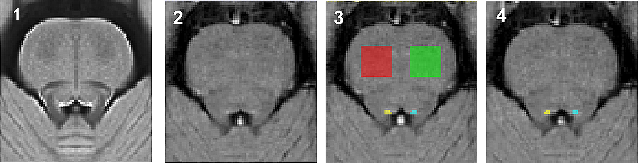
The total mean of the PPL values over trials was calculated for each channel for each participant. Higher PPL values show higher phase locking to the stimulus onset. The mean and SEM (standard error of the mean) of the resulting PPL values for the three different groups of participants are shown in Fig. 1.

PPL for healthy controls and aMCI and AD patients. PPL was calculated on channels A Fz B Cz C Pz for the non-frequent odor trials in the frequency range (39-41 Hz) in the gamma band. To assess the phase locking to the stimulus onset, the 0–0.7 s time interval after the stimulus onset was selected in each trial. A significant difference can be seen between the healthy group and the aMCI and AD groups in channels Fz and Cz (ns: not significant; *p < 0.05; **p < 0.01; ***p < 0.001. n = 15 Normal, n = 13 AD, n = 7 aMCI were used in this bar plot)

Synchronization of the gamma activity between different regions of the brain is another network-level mechanism that underlies memory and cognition (Jia et al. 2011). Amplitude coherence (Srinath and Ray 2014) is an indicator of spatial synchrony, which quantifies the synchronization of the amplitude fluctuations of two given signals. Amplitude coherence between channels Fz and Cz is defined as follows:

$$C_}}} \left( f \right) = \left| (A_}}} }} \left( f \right) - A_}_}}} }} \left( f \right))(A_}}} }} \left( f \right) - A_}_}}} }} \left( f \right))}} (A_}}} }} \left( f \right) - A_}_}}} }} \left( f \right))^ } \sqrt (A_}}} }} \left( f \right) - A_}_}}} }} \left( f \right))^ } }}} \right|,$$

where \(k\) is the number of trials and \(_\) is the absolute value of the Fast Fourier Transform (FFT) of the data record in each trial.

To calculate amplitude coherence, the 0–1 s post-stimulus interval was used and the slow-gamma oscillations (35–45 Hz) were extracted for each trial. \(__}}\) and \(__}}\) were calculated for each participant and \(_}\) was calculated for each frequency sample. Next, the values corresponding to the 35–45 Hz frequencies were averaged, yielding a mean \(_}\) value for each participant. The mean and SEM of these values for the three different groups of participants are plotted in Fig. 2.

Amplitude Coherence for healthy controls and aMCI and AD patients. Amplitude coherence was calculated between the A Fz–Cz, B Fz–Pz, and C Cz–Pz channel pairs for the non-frequent odor trials in the frequency range (35–45 Hz) in the gamma band. To measure the amplitude coherence, the 0–1 s time interval after the stimulus onset was selected in each trial. A significant difference can be seen between the AD group and the healthy and aMCI groups in Fz-Cz amplitude coherence (ns: not significant; *p < 0.05; **p < 0.01; ***p < 0.001. n = 15 Normal, n = 13 AD, n = 7 aMCI were used in this bar plot)

Phase-amplitude coupling (PAC) of different frequency bands in the brain has been suggested to be involved in the underlying mechanisms for different cognitive functions. Individuals diagnosed with AD show deficits of phase-amplitude coupling in their neural activity (Poza et al. 2017). It has been shown that the phase of slow oscillations in the brain [theta frequency band (4–8 Hz)] modulate the amplitude of higher frequency bands [slow gamma (35–45 Hz)], and that this neural mechanism is involved in performing memory-related tasks (Lega et al. 2014).

Several methods have been proposed for calculating the theta-gamma PAC. We used a recently introduced method called the time–frequency mean vector length (tf-MVL) (Munia and Aviyente 2019a, b). Unlike other methods that use Hilbert transform for extracting the phase of theta oscillations, tf-MVL uses the reduced interference distribution (RID)-Rihaczek method to simultaneously estimate the phase of the slow oscillations and the amplitude of the higher frequency oscillations. This method provides a more accurate estimate of the phase and amplitude of the signal as it does not depend on the parameters of filters to extract the theta and gamma components (Munia and Aviyente 2019a, b).

In this study, we compared the theta-gamma PAC for non-frequent odor trials on the Fz, Cz, and Pz channels. To this end, the data of each channel was normalized as z-score, setting the mean of each channel to zero and its standard deviation to 1. Next, the overall mean of the rest trials for each participant was subtracted from the average trial on each channel. Using the RID-Rihaczek distribution, the phase and amplitude of theta (4–8 Hz) and gamma (39–41 Hz) oscillations were extracted and the theta-gamma PAC value for each channel was calculated using the following formula:

$$} - }\,} = \left| \mathop \sum \limits_^ A_ e^ }} } \right|,$$

in which N is the length of the average trial on each channel, \(A\) is the amplitude of the sum of all the values corresponding to the slow-gamma frequency band in the (RID)-Rihaczek distribution, and \(\varphi\) is the angle of the sum of the values within the low frequency band in the time–frequency distribution.

The theta-gamma PAC was calculated for each participant and the mean and SEM of these values for channels Fz, Cz, and Pz are plotted in Fig. 3.

Theta-Gamma Phase Amplitude Coupling (PAC) for healthy controls and aMCI and AD patients. Theta (4–8 Hz)-gamma (39–41 Hz) PAC was calculated on channels A Fz, B Cz, and C Pz for the 0–2 s time interval after the stimulus onset in the frequent odor trials. A significant difference is observed between the aMCI group and both the healthy and AD groups for all three channels (ns: not significant; *p < 0.05; **p < 0.01; ***p < 0.001. n = 15 Normal, n = 13 AD, n = 7 aMCI were used in this bar plot)

Multiple binary SVM classifiers can be used for classifying data that consists of more than two groups. To classify the three groups of participants, two binary SVM classifiers were trained, both using as input the five features introduced in this section (PPL of channel Cz, amplitude coherence between channels Fz and Cz, and three PAC values for channels Fz, Cz, and Pz). The features were normalized before training the classifiers. One binary SVM classifier was trained for classifying healthy individuals and aMCI patients, and another for classifying aMCI and AD patients. For these two classifications, we separately trained a linear SVM classifier and a nonlinear SVM classifier using a radial basis function (RBF) kernel. While a nonlinear classifier may offer better performance through remapping of the features, using a linear classifier can demonstrate the intrinsic efficacy of the features regardless of the classification method. We also trained two binary Random Forest (RF) classifiers, one for classifying healthy individuals and aMCI patients, and another for classifying aMCI and AD patients.

Since the data used in these classifications were unbalanced, a stratified fivefold cross validation was performed to evaluate the performance of the classifiers. This allows for maintaining a fixed ratio between the number of positive and negative samples in all folds. Using this method, the mean and standard deviation of accuracy, precision, and recall were reported for all SVM and RF classifiers. The design of the classifiers and cross validation methods was conducted using the Python scikit-learn packageFootnote 1 (Pedregosa et al. 2011).

All results are expressed as mean ± \(\frac }}\), where \(n\) is the number of participants for each group, and \(\sigma\) is the standard deviation of the variable of interest. All p values were calculated using two-tailed t tests by MATLAB ttest2 function. Significance levels of 0.05, 0.01, and 0.001 were examined in each comparison.