Study sample and patient subgroups

A total of N = 40 male individuals (n = 11 pathological [problematic and addicted] gamers and n = 29 controls) were included in the current analyses. Initially, N = 83 participants enrolled in the study and completed baseline assessment. Of those, N = 40 returned for a second assessment after 12 months. N = 40 participants provided complete datasets. Participants were recruited between March 2016 and June 2019 (trial registration: DRKS 00009439). All procedures were carried out in accordance with the Declaration of Helsinki. The local ethics committee (application number 2014-602 N-MA) approved the study procedures and all participants provided informed written consent. Individuals were recruited via advertisement and outpatient care for pathological gamers in the Central Institute of Mental Health, Mannheim, Germany. Between the first (T1) and second assessment (T2), participants did not receive any specific intervention. The average time span between T1 and T2 was 396 days (SD = 67). Abstinence from substance use was monitored through drug urine screening at each assessment.

Participants were required to be aged between 18 and 27 years and had to be right-handed. Pathological gamers were excluded if they met any of the following exclusion criteria: (i) comorbid axis I disorders in the preceding year aside from nicotine-dependence and IGD, assessed using the Structured Clinical Interview for DSM-IV Axis I Disorders (SCID) [33] and the Assessment of Internet and Computer Game Addiction (AICA) [34]; (ii) treatment with psychotropic or anticonvulsive medications; (iii) severe neurological or physiological disease (such as, but not limited to stroke, aneurysm, dementia, epilepsy, liver cirrhosis); (iv) negative urine drug test on the day of assessment; or (v) contraindications for MRI scans (i.e., pace-makers, metal implants, tattoos).

Assessment

Participants underwent two assessment sessions, both including psychometric measures and fMRI. All participants completed questionnaires on (and after) the assessment day, including the Rosenberg Self-Esteem Scale [27], the Scale for Social Anxiety and Social Competence Deficits (SASKO; [15]), the Emotional Competence Questionnaire [26], and the Empathy Quotient [1]. Diagnosis of internet gaming addiction as well as problematic usage was evaluated with the Assessment of Internet and Computer game Addiction-Checklist (AICA-C > 13 for addictive usage and AICA-S > 6 and < 13 for problematic usage; [34]). After the first assessment, participants underwent interviews and filled out questionnaires every three months. After 12 months, participants were assessed via fMRI once again. Before the second scan, the exclusion criteria were reconfirmed. Participants were excluded if they had developed a comorbid axis I disorder (other than nicotine-dependence and IGD, in the preceding year); if they underwent treatment with psychotropic or anticonvulsive medications; or if they had suffered severe neurological or physiological disease in the preceding 12 months.

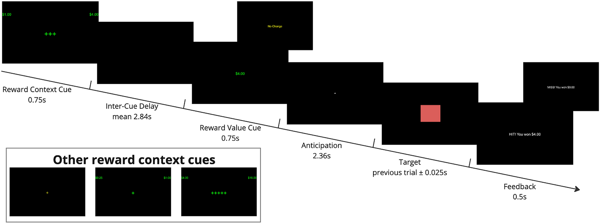
fMRI self-evaluation task

The paradigm comprised video clips of the participant themselves, an age-matched familiar person, and an unknown person. The task was programmed with the software Presentation Version 16.3 (Neurobehavioral Systems, Albany, Calif., USA). During a video session, participants and their close friend were asked to introduce themselves and talk about different topics related to their person. Four videos of each condition (self, a familiar, and an unknown person) comprised the following topics: (1) personal introduction (instruction: “Introduce yourself: name, age, family, etc.”); (2) positive character traits (instruction: “What are your personal strengths and hobbies?”); (3) personal values and expectations of other people (instruction: “What is important to you concerning your fellow humans?”); and (4) future goals (instruction: “Where do you see yourself in five years from now, what did you achieve?”). The videos, with duration of 15 s each, were recorded in advance with a Panasonic high-definition video camera (Type HC-V707) and converted using VSDS Free Video Editor software (Version 3).

The fMRI paradigm was conducted in a block design. Each paradigm block consisted of a video clip regarding one topic from one specific condition. All blocks were presented in a randomized order. Every participant watched 12 video clips in total (three conditions comprising four videos each). Each video clip was followed by a fixation cross (two seconds) and a distractor (calculation task with a maximum duration of 13 s), where participants had to move the cursor to select an answer. Then, another fixation cross appeared before the subsequent video clip began. The distractor was used to create distance between the previous videos’ content. The total paradigm took a minimum of four and a maximum of 8 min, depending on how fast the participants solved the calculation task (see Fig. 1).

Fig. 1

Depiction of the self-evaluation block-design paradigm

MRI acquisition

MRI data acquisition was performed on a 3.0 Tesla MR scanner (SIEMENS MAGNETOM Trio) with a standard multi-channel receiver head coil (12-channel). During the functional self-concept MRI task, 205 volumes were acquired by applying a T2*-weighted echo-planar imaging (EPI) sequence [repetition time (TR) = 2410 ms, echo time (TE) = 25 ms, flip angle (FA) = 80°, field of view (FOV) = 192 mm × 192 mm, matrix size 64 × 64, 42 slices, slice thickness = 2.00 mm, distance factor = 50%, and voxel size = 3 × 3 × 2 mm]. Three-dimensional T1-weighted structural images (Magnetization Prepared Rapid Acquisition Gradient Echo, MPRAGE) were collected over 8 min. The T1-weighted anatomical scans comprised 192 sagittal slices (flip angle: 9˚; repetition time: 2.3 ms; echo time: 3.03 ms; field of view 256 × 256; voxel size, 1 mm × 1 mm × 1 mm). The automated Siemens Multi-Angle Projection (MAP) Shim corrected magnetic field inhomogeneity. Presentation software (Version 16.3, Neurobehavioral Systems, Inc., Albany, CA, USA) was used for both the registration of scanner triggers and the recording of behavioral responses. All participants viewed the video clips through a tilted mirror placed above their heads. During the assessment, the test persons wore foam ear plugs and headphones. Prior to the assessment, participants underwent a hearing test to adjust the sound of the video clips if necessary. After completion of the scan, participants were asked to rate the sound quality of the videos on a scale from 0 to 10. One patient, who rated the sound quality under 7, was excluded from the analyses.

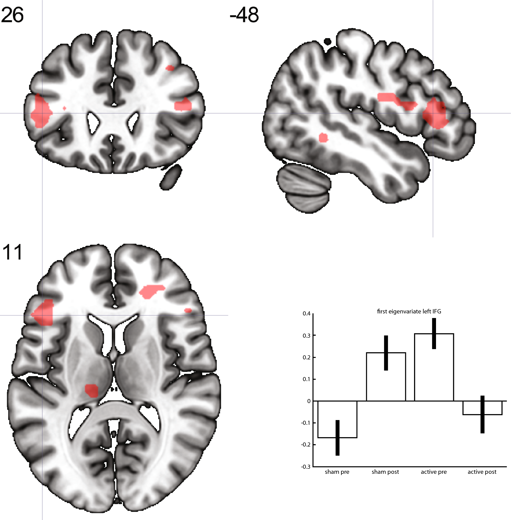
fMRI pre-processing and statistical analyses

The functional images were pre-processed according to standard procedures implemented in the statistical parametric mapping software for Matlab (SPM, Wellcome Department of Cognitive Neurology, London, UK) version 12. The first five scans of every measurement were discarded to avoid artifacts due to magnetic saturation. We conducted slice time correction, followed by spatial realignment and unwarping. A phase map correction was applied to correct geometric distortions, using a voxel displacement map that was computed from a gray field mapping sequence using the VDM utility in SPM12. Movement correction was conducted using standard SPM12 parameters and images were normalized to the standard tissue probability template provided in SPM12. Smoothing was conducted using an isotropic Gaussian kernel for group analysis (8 mm Full Width at Half Maximum). The following procedures were carried out to assess the quality of pre-processed functional MRI data. Motion correction and realignment parameters, as well as results from the normalization procedure, were assessed by two independent trained members of the study team. Datasets of participants were excluded if the spatial realignment or movement correction parameters indicated excessive motion (> 3 degrees of rotation or > 3 mm movement in any axis) or if visual inspection indicated poor fitting to the standard TPM template. The first-level statistics were computed for each participant, modelling the different experimental conditions: (i) self, (ii) familiar person, (iii) unknown person, and (iv) distractor task in a generalized linear model including six motion parameters as covariates. The general view of the self-concept is that of a stable cognitive representation (i.e., knowledge system and beliefs) about one’s subjective self in comparison to an ideal self, the latter of which is formed by the environment. In line with this view, the neural correlates of the self-concept were operationalized by subtracting brain activation during the presentation of videos of oneself from the brain activation during the presentation of videos of familiar and unknown persons (i.e., self > familiar person and unknown person). Thus, apart from the contrast images for (i) self vs. implicit baseline; (ii) familiar person vs. implicit baseline; (iii) unknown person vs. implicit baseline; (iv) distractor condition vs. implicit baseline; and (v) self vs. familiar and unknown person. The contrast between self and familiar person + unknown person was computed using the contrast weights (2 -1 -1 0) .

Previous studies suggested that difference measures suffer from low inherent reliability when the constituting conditions are correlated [11]. Hence, we also estimated reliability separately for the “self”, “familiar other”, and “unknown other” contrast conditions.

Analyses of self-concept-related measures

We tested the stability of self-concept measures (i.e., with SASKO, the Emotional Competence Questionnaire, the Rosenberg Self-Esteem Scale, and the Empathy Quotient) by assessing differences between the first and second experimental session (t tests for dependent samples) for pathological (problematic and addicted) gamers and healthy controls separately. Furthermore, we assessed test–retest reliability of self-concept measures by computing the intraclass correlation coefficient between the first and second session.

Analyses of group-level fMRI activation

On a group level, imaging data were analyzed using full factorial models with the factor time (first and second scan) to assess the congruence of task effects on the group-level brain activation over time. This was accomplished by determining brain areas that show higher brain activation in response to viewing videos of the own person compared to brain activation when viewing videos of familiar and foreign persons (contrast: “self > familiar and unknown person”). In addition, group-level brain activation patterns were analyzed for the constituting task conditions separately (i.e., responses to videos of the “self”); a familiar person (contrast: “familiar person”); and an unknown person (contrast: “unknown person”) at each time point. We applied a whole-brain family-wise error rate correction of pFWE < 0.05 at the cluster level to correct for multiple comparisons.

Reliability measures

To assess longitudinal test–retest reliability of the self-evaluation fMRI task, we computed global and local measures of reliability. All reliability analyses were conducted using the fmreli toolbox for SPM12 [8]. Individual contrast images of the different task conditions served as input for the reliability analyses. Dice and Jaccard coefficients were analyzed within the framework of an ANOVA with the contrast condition set as four-level within-subject factor (i). self; (ii). familiar person; (iii). unknown person; (iv). self > familiar + unknown person and the experimental group set as two-level between-subject factor [(i). healthy individuals; (ii). IGD].

Intraclass correlation coefficient

Voxel-wise reliability of each contrast condition was estimated by computing the intraclass correlation coefficient (ICC) between the first and second assessment points. The ICC tests whether the magnitude of brain activation in each voxel is stable between the first and the second fMRI scan. Fleiss (1986) proposed that ICCs lower than 0.4 indicate poor reliability; ICCs between 0.4 and 0.6 indicate fair reliability; ICCs between 0.6 and 0.75 indicate good reliability; and ICCs with values higher than 0.75 indicate well to excellent reliability [6]. The ICC sets within-subject variance (σ2within) in relation to between-subject variance (σ2between). The ICC(3,1)-type was proposed as being the most appropriate for assessing single site longitudinal fMRI datasets [23]. Hence, we used the ICC(3,1)-type [28], defined as:

$$ICC = \frac_}}} - \sigma^_}}} } \right)}}_}}} + \sigma^_}}} } \right)}}.$$

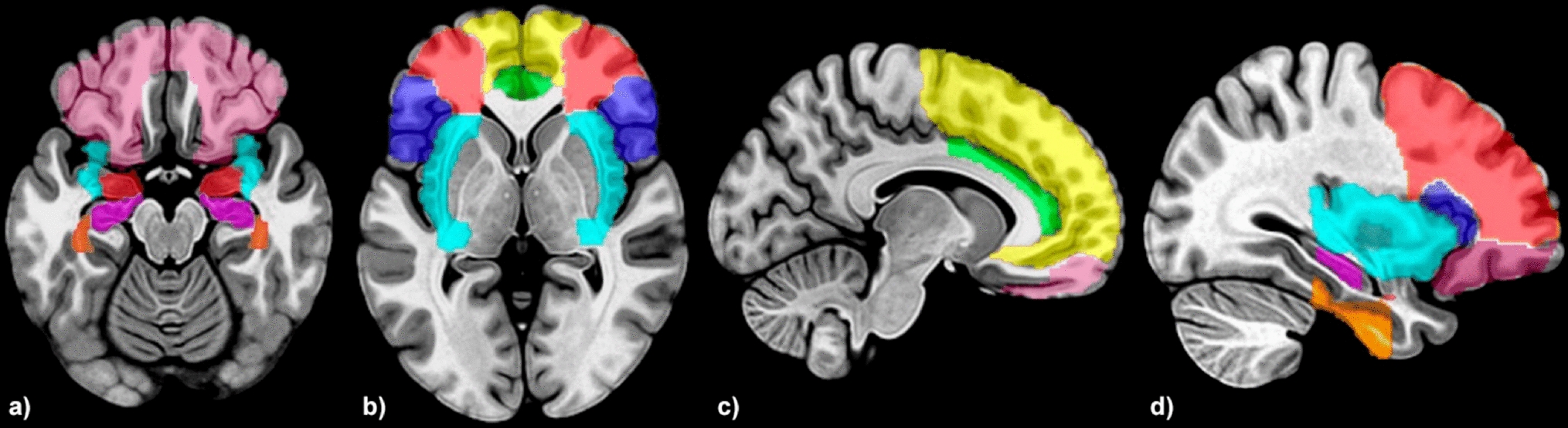
ICC values were computed for the contrasts of “self”, “familiar person”, “unknown person”, and the contrasts “self > familiar and unknown person”. We computed ICCs for every brain voxel and generated thresholded ICC brain maps to identify brain areas that show good (ICC > 0.6) and good to excellent (ICC > 0.75) reliability. Furthermore, we computed additional atlas-based mean ICC values for a standard set of anatomical brain regions (see below).

Similarity

Similarities in the fMRI activation maps from the first and second scans were determined. The analysis captures the resemblance of two brain activation maps based on the alignment of high vs. low brain activation values across the brain. The authors of the fmreli toolbox propose that this method could be used to quantify within-subject and between-subject similarities of brain activation without requiring an a priori (and potentially arbitrary) statistical threshold. A high within-subject similarity supports the notion that individuals can be re-identified based on their neural brain activation patterns. The resulting coefficients are correlation coefficients that range from a “perfect” negative relationship (− 1.00) to a “perfect” positive relationship (1.00). In the past, studies have suggested that subjects can be successfully identified based on their neural activation pattern if the within-subject similarity exceeds all between-subject association coefficients of the same participant [5, 8]. The similarity analyses, therefore, complement the computation of the ICC, which allow inferences on a group level, providing additional information on the stability and resemblance of brain activation at an individual participant level.

Pearson’s correlation

We computed the mean voxel-wise Pearson’s correlation coefficients between the “self”, “familiar other”, and “unknown other” contrast conditions using the procedures provided in the fmreli toolbox. This step was taken to assess the correlation between the different task condition contrasts. This is important due to the fact that the reliability of a contrast between two conditions is limited in the case of high correlation between the activation patterns of the constituting contrast conditions.

Jaccard and dice coefficients

The modified Jaccard coefficient is a commonly used measure in fMRI reliability studies. It can be interpreted as the percentage of overlapping significant voxels above a predefined threshold (e.g., p < 0.001) within all significant voxels. The Jaccard coefficient is defined as the ratio of intersection between the number of three-dimensional image voxels, which were found to be activated in the first fMRI assessment (A) and the replication (B), divided by the size of the union of the voxel sets of A and B [12, 20].

$$}\left( \right) = \frac \right|}} \right|}} = \frac \right|}} \right|}}.$$

Another measure of global reliability or overlap between super-threshold voxels is the Dice coefficient. It is calculated as the number of super-threshold voxels that overlap between sessions A and B (see above) divided by the average number of significant voxels across sessions A and B (see above):

$$}\left( \right) = \frac \right|}}.$$

Both, Jaccard and Dice coefficients range from no overlap (0) to perfect overlap (1) between super-threshold voxels; however, currently there is no consensus on specific values or cut-offs that would differentiate between “poor” and “good” values [2]. In accordance with previous studies, the current analyses used a threshold of p < 0.001. Jaccard and Dice coefficients were determined for every patient by comparing the baseline and the second fMRI results for the different contrast images. Resulting values were exported into the IBM SPSS statistics software (version 25.0) and effects of contrast conditions were tested using a repeated measures analysis of variance model with contrast condition as within-subject factor.

Atlas- and ROI-based summary measures

To facilitate the assessment of local differences in reliability, we computed the mean ICC for N = 116 anatomical regions, specified in the automatic anatomic labeling (AAL) atlas [30]. ICC values were extracted from the ROIs using the data extraction routine of the MarsBar software package (http://marsbar.sourceforge.net/); then, these data were exported into the IBM SPSS statistics software (version 25.0) for further analyses.