The uniform positron range distribution of 124I was simulated using GATE 9.0 (GEANT4 10.06.p02). The simulation setup consisted of a point source with a radius of 5 nm centered in a uniform phantom with a radius of 30 cm. For the phantom material, three settings were simulated bone material (mass density 1.92 g/cm3), water (1.00 g/cm3), and lung equivalent material (0.26 g/cm3). The predefined “empenelope” physics list was used. The initial activity of 124I was 10 MBq and the emission and annihilation coordinates were recorded for 20 M annihilation events. From the recorded data, the 3D PR distribution was generated by mapping the distribution to a 3D matrix. The size of the kernel (11 × 11 × 11 voxels) was chosen based on the voxel size of the Siemens mCT PET/CT system (2 × 2 × 2 mm3) (Siemens Medical Solutions Inc., Knoxville, TN, USA) [20] and the maximum PR in water for 124I (~ 10 mm), since the use of larger kernels is leading to artifacts [14].

For each voxel of the investigated object, spatially variant and tissue-dependent PR kernels based on the underlying material distribution were created as described before [14]. In short, the attenuation map was segmented into a material map containing lung, soft tissue, and bone. Regions containing air were treated as lung material. Then, for every voxel, PR kernels were generated by combining pre-calculated uniform PR kernels for lung, water, and bone from GATE Monte Carlo simulations.

The PR correction was implemented into the vendor-based software in combination with OSEM and PSF algorithms as an additional PR-dependent PSF applied in image space. This was done as full implementation and, in addition, in a simplified version applying the PR-dependent blurring only before the forward projector of the reconstruction algorithm, as suggested by [19] to reduce computational demand.

The standard OSEM algorithm taken as the basis can be written as:

$$f_^ = \frac^ }} \in S^ }} j} } }}\sum_ }} a_ \frac }} a_ f_^ }}$$

(1)

where fjn+1 is the next image estimate of voxel j based on the current image estimate fkn. The measured projection data is mi. The system matrix describing the probability that the emission from voxel j will be detected along the line of response (LOR) i is given by Aij = (aij)IxJ. Only a subset Sn of the data was used in each update. Of note: for simplification, the random and scatter are not included in this description. The system matrix can be factorized to account for the finite resolution effects, in our case the positron range effect by matrix H = (hj’j)JxJ, a matrix X = (xij)IxJ expressing the intersection length and a matrix W = (wii)IxI describing the photon attenuation and geometrical sensitivity variations. Thus, the system matrix can be written as:

Combining Eq. (1) and Eq. (2), the OSEM algorithm with PRC correction can be written as [14]:

$$_^=\frac_^}___^}__}___^}_\frac_}_____^}$$

(3)

This method is referred to as “PRC” in this work. Since PRC is computationally highly expensive, a simplified version of the PRC implementation was suggested in previous studies [18, 21], where the PR kernels are applied to the current image estimate as a convolution in image space before the forward projection. In this way, Eq. (1) can be written as:

$$f_^ = \frac^ }} \in S^ }} j} } }}\sum_ }} a_ \frac }} a_ f_^ }} }}$$

(4)

where \(f_^ }}\) is the current image estimate blurred with the spatially variant and tissue-dependent PR kernel (\(\rho\)) calculated for the given voxel [19]:

$$f_^ }} = f \otimes \rho = \frac f_ - \rho_ }}^} \rho_ }}$$

(5)

This method is referred to as “PRC simplified” in this study. Both PRC methods (PRC and PRC simplified) together with the generated PR kernels were implemented into the Siemens e7tools (Siemens Medical Solutions USA, Inc., Knoxville, TN, USA) image reconstruction framework using MATLAB R2019a (MathWorks Inc, USA). The image reconstructions with both PRC implementations were performed with both OSEM and PSF corrected OSEM (PSF): OSEM algorithm with PR implemented in the forward projection only (OSEM+PRC simplified), OSEM with PRC implemented in both forward- and back-projection (OSEM+PRC). The same naming convention was used for PSF reconstructions (PSF+PRC simplified and PSF+PRC).

All reconstructions were done with 1–10 iterations and 12 subsets, except the reconstruction for which PSF was combined with PRC in the back-projection (PSF+PRC). In this case, image reconstructions were performed with 1–20 iterations and 12 subsets. The image size was 400 × 400 x 109 voxels, with a voxel size of 2 × 2 × 2 mm3. All emission data was corrected for attenuation, normalization, scatter, and randoms. The time-of-flight (TOF) information was included and no post-reconstruction filters were applied.

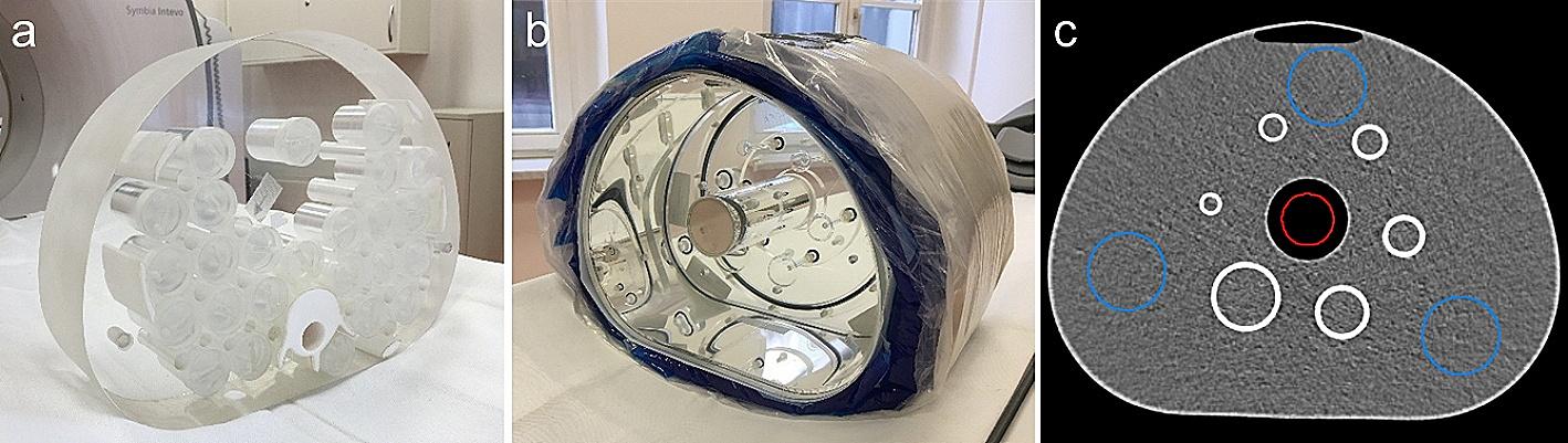
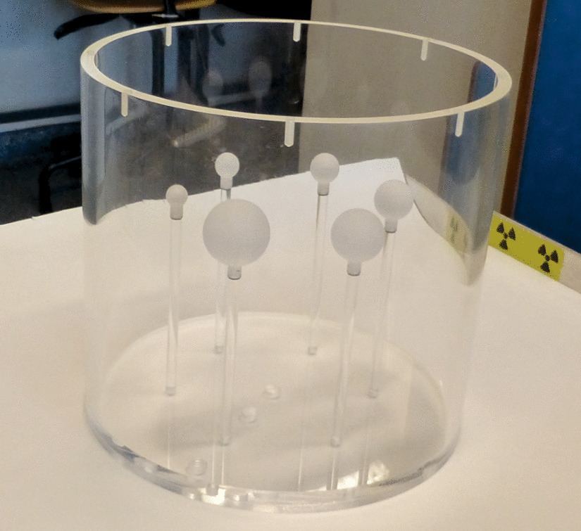
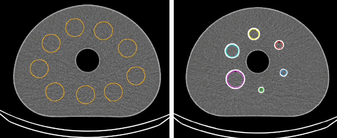
The PRC implementations were tested and compared by means of contrast, noise, and convergence properties using the standard “NEMA Image Quality (IQ)” phantom, a modified NEMQ IQ phantom with changed hot spheres referred to as “Small-tumor” phantom and a “Bone–lung” phantom. Of note, the NEMA IQ phantom simulates hot lesions embedded in soft tissue (water) only (Additional file 1: Fig. S1a). The Small-tumor phantom is a specially-modified phantom using the housing of the NEMA IQ phantom, with fillable spheres with diameters of 3.7, 4.8, 6.5, 7.7, 8.9, and 9.7 mm (Additional file 1: Fig. S1b). The dedicated Bone–lung phantom simulates hot lesions embedded in lung and bone mimicking material, and thus, allows a comparison of the PRCs in a tissue-dependent environment (Additional file 1: Fig. S1c). All phantom acquisitions were performed at the University Clinic Essen, Germany, using the Siemens mCT PET/CT system [20].

In the NEMA IQ phantom, all the spheres (diameter of 10, 13, 17, 22, 28, and 37 mm) were filled with a 124I activity concentration of 30 kBq/ml, and the background region was filled with an activity concentration of 6 kBq/ml. The emission acquisition time was 60 min. The phantom was positioned with the centers of the spheres in the center of FOV. For the evaluation, 12 volume-of-interests (VOIs) were used in the background region (each with a diameter of 37 mm) and 6 individual VOIs covering every sphere (with the diameter corresponding to the sphere size) (Additional file 1: Fig. S1d). For placing the background VOIs, the center of the FOV slice was selected, where all the spheres are centered as well. The reconstructed images were evaluated for contrast recovery calculated as:

$$}\; } = \frac}_}}} }}}_}}} }}}}}\;}}}$$

(6)

where the mean value in the background was calculated as the mean overall VOIs.

Image noise was defined in percentage following the guidelines of EFOMP [22]:

$$} = \frac}_}}} }}}_}}} }}*100$$

(7)

The convergence of the investigated reconstruction algorithms in combination with the various PRC implementations was assessed by plotting the contrast recovery vs. noise and how fast contrast recovery and noise is changing with each iteration [14, 23]. For a direct comparison of the reconstructed images, the reconstruction settings were selected to match a 10% background noise as defined as a clinical acceptable noise level as gained from phantom scans [22].

The Small-tumor phantom was filled with a 124I activity concentration of 25 kBq/ml in the hot lesions and a background activity of 1.2 kBq/ml leading to a signal-to-noise ratio of 20:1. The acquisition time was 30 min [7]. The reconstructed images were evaluated for contrast recovery (Eq. 5) and image noise (Eq. 6) by defining 10 VOIs in the background region (diameter of 20 mm) and individual VOIs for every sphere (with the diameter corresponding to the sphere size) (Additional file 1: Fig. S1e).

The Bone–lung phantom was composed of 3 different cylinders (each with a diameter of 50 mm) made of different materials (lung with -800 HU, bone with 500 HU, and 1000 HU) that are housed within the standard NEMA IQ phantom [24]. Within every cold cylinder, two fillable spheres were inserted, one with a diameter of 8.5 mm and one with 19.4 mm. The spheres were filled with a 124I activity concentration of 30 kBq/ml and the background with 6 kBq/ml. Similar to the NEMA IQ evaluations, 6 background VOIs (diameter of 37 mm) and VOIs covering the hot spheres (diameter of 8.5 and 19.4 mm) were defined (Additional file 1: Fig. S1f). The acquisition time was 60 min, and the reconstructed images were evaluated for contrast recovery (Eq. 5) and noise (Eq. 6).