Restricting DNAm array probes to the most variable sites could improve power in association studies whilst minimising array content. We show that this approach hampers variance component analyses and that phenotypes with strong epigenetic correlates are the most robust to changes in the number of available probes. Further, loci with an mQTL and with intermediate DNAm levels are central to epigenetic predictions of clinically relevant phenotypes. Our results provide methodological considerations towards the goal of selecting reduced array content from existing methylation microarrays, which can afford more cost-effective methylomic analyses in large-scale population biobanks. However, substituting or removing probes results in alterations to chip design and possibly the background physiochemical properties of the array. Therefore, it is not appropriate to assess the transferability of the present findings to other, related platforms. Nevertheless, our data demonstrate that strategies aiming to minimise arrays using fewer probes must carefully select CpG or probe content in order to maximise epigenetic predictions of human traits.

MethodsStudy cohort

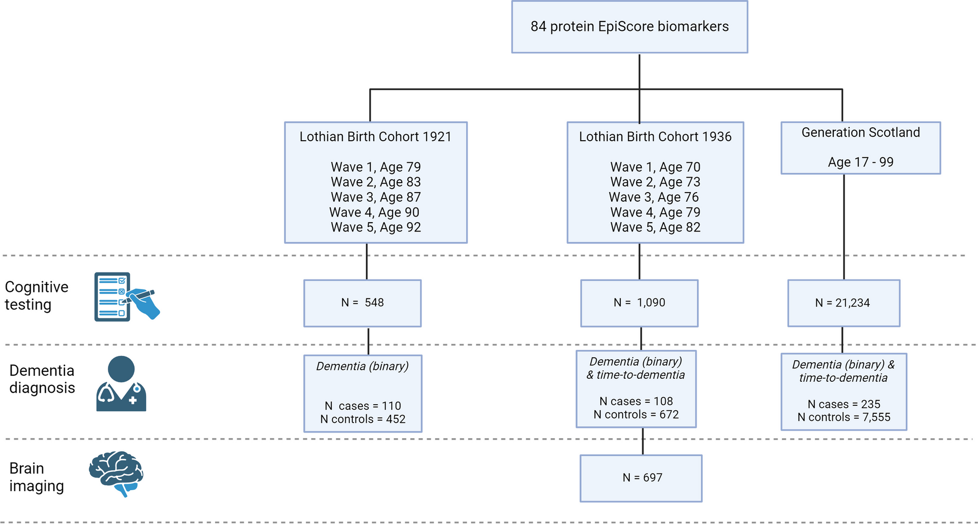
Details of Generation Scotland (GS) have been described previously [26, 27]. GS is a family-based, genetic epidemiology cohort that consists of 24,084 volunteers. There were 5573 families with a median size of 3 members (interquartile range = 2–5 members, excluding 1400 singletons). Genome-wide DNAm was profiled using blood samples from GS baseline (2006–2011). DNAm was processed in two separate sets of 5200 (2016) and 4585 samples (2019) [35].

Preparation of DNA methylation data

DNAm was measured using the Infinium MethylationEPIC BeadChip at the Wellcome Clinical Research Facility, Western General Hospital, Edinburgh. Methylation typing in the first set (n = 5200) and the second set (n = 4585) was performed using 31 batches each. Full details on the processing of DNAm data are available in Additional file 3. Poor-performing and sex chromosome probes were excluded, leaving 760,943 and 758,332 probes in the first and second sets, respectively. Participants with unreliable self-report questionnaire data (self-reported 'yes' for all diseases in the questionnaire), saliva samples and possible XXY genotypes were excluded, leaving 5087 and 4450 samples in the first and second set, respectively. In the first set, there were 2578 unrelated individuals (common SNP GRM-based relatedness < 0.05). In the second set, all 4450 individuals were unrelated to one another. Individuals in the first set were also unrelated to those in the second set. The second set (profiled in 2019) was chosen for OSCA models and as the training sample in DNAm-based prediction analyses given its larger sample size (n = 4450). Unrelated individuals from the first set (profiled in 2016) formed the test sample in DNAm-based prediction analyses (n = 2578). Linear regression models were used to correct probe Beta-values for age, sex and batch effects separately within the training (n = 4450) and test samples (n = 2578).

Identification of variable probes in blood

There were 758,332 sites in the training sample (n = 4450) following quality control. First, we restricted sites to those that are common to the 450K and EPIC arrays to allow for generalisability to other epigenetic studies (n = 398,624 probes). We excluded loci that were predicted to cross-hybridise and those with polymorphisms at the target site, which can alter probe binding (nprobe = 4970 excluded, 393,654 remaining) [36, 37]. These 393,654 probes represented the reference set in our analyses, which we defined as ‘all available probes’.

We then defined a set of criteria to identify variable probes within blood tissue, specifically. First, we removed sites that are hypo- or hypermethylated in the sample (i.e. mean Beta-value ≤ 10% or ≥ 90%, respectively, nprobe = 144,150 excluded). Hypo- and hypermethylated sites had a mean SD of 0.01 (range = [0.002, 0.13]). Probes with mean Beta-values between 10 and 90% (nprobe = 249,504) had a mean SD of 0.03 (range = [0.008, 0.33]). Second, we excluded 133,758 probes that overlapped with known blood-based mQTLs (GoDMC [16], P value < 5 × 10–8). There were 115,746 remaining sites, which represented the ‘variable non-mQTL probes’ subset. We then extracted the 50,000, 20,000 and 10,000 non-mQTL probes with the highest SDs (mean SD = 0.04, 0.05, 0.06, respectively, Additional file 1: Table S10).

Preparation of phenotypic data

Eighteen traits were considered in our analyses. Full details on phenotype preparation are detailed in Additional file 3. The seventeen biochemical and complex traits (excluding chronological age) were trimmed for outliers (i.e. values that were ± 4 SDs away from the mean). Fifteen phenotypes (excluding FEV and FVC) were regressed on age, age-squared and sex. FEV and FVC were regressed on age, age-squared, sex and height (in cm). Correlation structures for raw (i.e. unadjusted) and residualised phenotypes are shown in Additional file 2: Fig. S3 and S4, respectively. For age models, DNAm and chronological age (in years) were unadjusted. Residualised phenotypes were entered as dependent variables in OSCA or penalised regression models.

Variance component analyses

OSCA software was used to estimate the proportion of phenotypic variance in eighteen traits captured by DNAm in the training sample (n ≤ 4450) [10]. In this method, an omic-data-based relationship matrix (ORM) describes the co-variance matrix between standardised probe values across all individuals in a given data set. Here, the ORM was derived from age-, sex- and batch-adjusted Illumina probe data and is fitted as a random effect component in mixed linear models. Phenotypes were pre-corrected for covariates as described in the previous section. Restricted maximum likelihood (REML) was applied to estimate the variance components, i.e. the amount of phenotypic variance captured by all DNAm probes used to build an ORM. We developed 18 ORMs in total reflecting all probe sets described: (i) one for ‘all available probes’, (ii) four for the ‘variable non-mQTL probe’ sets, (iii) five for ‘variable mQTL probe’ sets, (iv) five for hypo- and hypermethylated probe sets and (v) three for EWAS Catalog probes. The probe sets are outlined in full in Additional file 1: Table S10.

The variance component estimates are analogous, but not equivalent, to SNP-based heritability estimates [38, 39]. However, SNP-based heritability estimates have an inference of association through causality. The epigenetic variance component estimates could reflect both cause and consequence with respect to the phenotype and are not readily extended to other samples with different background characteristics. REML estimates served as important within-sample variance estimates in the present study, allowing us to assess the impact of the number of probes used to build an ORM, and their properties, on the amount of phenotypic variance captured by probe values. We then applied penalised regression models to build linear DNAm-based predictors of the phenotypes in the training sample. We carried out these analyses in order to assess the relative predictive performances of the probe sets when applied to a separate test sample (n < 2578), described below.

LASSO regression and prediction analyses

Least absolute shrinkage and selector operator (LASSO) regression was used to build DNAm-based predictors of eighteen phenotypes. The R package biglasso [40] was implemented and the training sample included ≤ 4450 participants. The mixing parameter (alpha) was set to 1 and tenfold cross-validation was applied. The model with the lambda value that corresponded to the minimum mean cross-validated error was selected. Epigenetic scores for traits were derived by applying coefficients from this model to corresponding probes in the test sample (n = 2578). This method takes into account the correlation structure between probes, but only selects a weighted additive combination of probes that are informative for predicting a given trait. Therefore, epigenetic predictors or methylation risk scores are broadly analogous to polygenic risk scores, which often show R2 estimates that fall far below SNP-based heritability estimates [41]. Here, our goal was to compare the relative predictive performances of probe sets in an out-of-sample context, distinct from the earlier approach of estimating variance components within the training sample alone.

Linear regression models were used to test for associations between DNAm-based predictors (i.e. epigenetic scores) for the eighteen traits and their corresponding phenotypic values in the test sample. The incremental r-squared (R2) was calculated by subtracting the R2 of the full model from that of the null model (shown below). For the FEV and FVC predictors, height was included as an additional covariate in both models. For the age predictors, the R2 value pertained to that of the epigenetic score without further covariates.

$$Null \, model:}\sim } + }$$

$$Full \, model:}\sim } + } + }$$

Sub-sampling analyses

We tested whether variance components and incremental R2 estimates from probe sets were significantly different from those expected by chance. For OSCA estimates, we generated 1,000 sub-samples of 115,746, 50,000, 20,000 and 10,000 probes (to match the primary subsets of non-mQTL probes tested in our analyses). The sub-sampled sets were sampled from ‘all available probes’ (nprobe = 393,654). We also generated 100 sub-samples of 115,746, 50,000, 20,000 and 10,000 probes, and not 1,000 sub-samples, for LASSO regression in order to lessen the computational burden.

We tested whether highly variable probes were significantly over-represented or under-represented for genomic and epigenomic annotations. Annotations were derived from the IlluminaHumanMethylationEPICanno.ilm10b4.hg19 package in R [42]. Annotations for the most variable primary subset (i.e. 10,000 non-mQTL probes) were compared against 1,000 sub-samples of non-mQTL CpGs with an equal number of probes. Here, probes were sub-sampled from the ‘variable non-mQTL probes’ set (nprobe = 115,746) and not from ‘all available probes’ (nprobe = 393,654) as the latter contains probes with and without mQTLs, which show different genetic architectures [16].

Comparisons of methylation QTL status and mean Beta-values

In addition to non-mQTL subsets (with mean Beta-values between 10 and 90%), we tested two further classes of probes. First, we considered probes with a reported mQTL from GoDMC (P < 5 × 10–8) that had mean Beta-values between 10 and 90% (nprobe = 133,758) [16]. Second, we considered all hypo- or hypermethylated probes (Beta-value ≤ 10% or ≥ 90%, nprobe = 144,150). We tested the performances of the 115,746, 50,000, 20,000 and 10,000 most variable probes from each of these three classes.

We also repeated REML and LASSO regression using EWAS Catalog probes [43]. EWAS Catalog probes contained sites with an mQTL, sites without an mQTL and hypo- and hypermethylated sites. We restricted EWAS Catalog probes to those with P < 3.6 × 10–8 [44] and those reported in studies with sample sizes > 1000. We also excluded studies related to chronological age due to the very large number of sites implicated and alsothose in which Generation Scotland contributed to analyses. There were 100 studies that passed inclusion criteria with 47,093 unique probes. Of these, 38,853 probes overlapped with ‘all available probes’ used in our analyses (nprobe = 393,654). To allow for comparison to other subsets, the 20,000 and 10,000 most variable EWAS Catalog probes (nprobe = 38,853) were extracted.