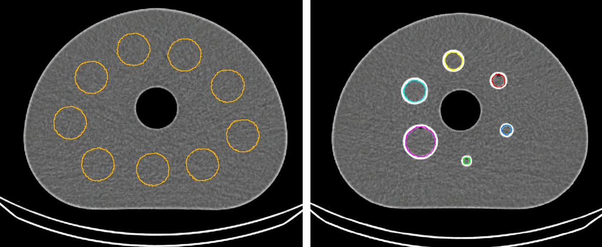
An overview of the three different regions in the NEMA NU-4-inspired phantom with and without PRC is shown in Fig. 2. In the uniform area, the border between air and the phantom was more blurred with no PRC compared to the two PRC reconstructions. TDSV had a slight halo effect around the edges, also known as a Gibbs artifact [17]. In the left cylinder in the cold region (water), a great amount of spillover was present with no PRC compared to both PRC images. The spillover was more similar for all methods in the right air-filled cylinder, but the rod was still better delineated in the PRC images. In the rod region, the PRC reconstructions had more visible rods for 3–5 mm compared to the reconstruction without PRC, where the rods were more blurred.

Axial view of the NEMA NU-4 phantom for the uniform, cold and rod region, shown for 40 iterations with no PRC, TD 2 and TDSV 41. All images are shown with the same intensity window. PRC = positron range correction; TD = tissue-dependent; TDSV = tissue-dependent spatially variant

The results are shown in Fig. 3. Overall, the no PRC method had a lower %SD until about 25 iterations, where the PRC curve superseded the no PRC curve. For all methods, the %SD kept increasing, but the PRC curves had a greater slope than no PRC, where TD 1 and 2 and TDSV 21 were very similar, while TDSV 41 had a slightly greater slope and also a higher offset than the other PRC methods.

Percent standard deviation shown for 1–100 iterations with no PRC, TD 1 and 2, and TDSV 21 and 41. Abbreviations as in Fig. 2

The results are presented in Fig. 4 and Table 1. With no PRC, the SOR in the air-filled cylinder converged to about 0.1, while all PRC methods converged close to 0 after about 40 iterations. TD 2 converged slightly slower than the other PRC methods. The standard deviation (SD) of SOR in air converged to about 0.025 for no PRC and to 0 for all PRC methods after about 60 iterations.

SOR shown for 1–100 iterations with no PRC, TD 1 and 2, and TDSV 21 and 41. SOR = spillover ratio, other abbreviations as in Fig. 2

In the water-filled cylinder, no PRC converged to about 0.4 after 30 iterations, while the SOR for all PRC methods kept decreasing. TD 1 and 2, and TDSV 21 reached about 0.05 after 100 iterations while TDSV 41 reached around 0. The SD of SOR in water increased with more iterations for no PRC, while it kept decreasing for all the PRC methods. It decreased faster for TDSV 41 compared to the other PRC methods.

The results are shown in Fig. 5 and Table 1. For no PRC, the RC converged after 10 iterations and was between 0.1 and 0.5. PRC mainly had an effect on the RC for the 3–5 mm rods, which all exceeded 1. The RC graphs for TD 1 and 2, and TDSV 21 were essentially identical, while the RC for TDSV 41 increased faster for the 3–5 mm rods. The SDs for no PRC were smaller than for the PRC methods.

RC shown for 1–100 iterations with no PRC, TD 1 and 2, and TDSV 21 and 41. RC = recovery coefficient; SD = standard deviation, other abbreviations as in Fig. 2

The effect of post-filtering with a Butterworth filter (order 10, cutoff 0.2) is shown in Figs. 9, 10, 11 and 12 and in Table 3. Filtering reduced the noise for %SD and RC, as well as preventing the RCs from rising much higher than 1, while the SOR is mostly unchanged. The Butterworth filter reduced the noise more for the TD methods than for the TDSV.

Figure 6 shows the PET/CT for the cardiac phantom with no PRC in 3 planes (axial, coronal and sagittal) and the line profiles of the phantom. The lumen of left and right ventricle could not be clearly discerned from the ventricular wall due to the amount of spillover on neither the PET image (Fig. 14) nor the line profiles (Fig. 6B, C). More than 30 iterations did not improve the image quality (data not shown).

a PET image with no PRC and CT of the cardiac phantom, shown in the axial, coronal and sagittal plane for 30 iterations. The image was interpolated with B-splines. The blue crosshairs indicate where the coronal and sagittal line profiles were shown. Line profiles for the b Coronal c Sagittal planes. The black lines show the placement of the right ventricular wall (leftmost) and the left ventricular walls (two to the right). Bq = Becquerel; iter = iterations; PET = positron emission tomography; CT = computed tomography, other abbreviations as in Fig. 2

The results of TD 2 PRC are shown in Fig. 13 for 20, 40, 80 iterations with their line profiles, 80 iterations filtered with a Butterworth filter and an 18Fluorodeoxyglucose (FDG) scan of the phantom for comparison. Figure 13B and 7C show the line profiles. Only TD 2 is shown, as TD 1 gave identical images (Table 2).

Compared to no PRC (Fig. 6), the right ventricular wall and lumen were clearly distinguishable. The spillover into the lumen of the left ventricle was almost eliminated at 80 iterations (Fig. 13B, C). The right ventricular wall and lumen could be seen after 80 iterations, but were not clearly delineated compared to the FDG scan. The difference in peak activity of the septum and lateral ventricular wall increased with more iterations (Fig. 13B), while it stayed similar in the anterior and inferior left ventricular wall (Fig. 13C).

More iterations also resulted in a more speckled PET image (Fig. 13A), which could be moothed by post-filtering the image with a Butterworth filter. Compared with the FDG scan, the FWHM and FWTM of the left ventricular wall (Table 2) improved substantially compared to no PRC.

The results of TDSV 41 (Fig. 7) were similar to those of TD 2, with a few differences. At 40 and 80 iterations, the lumen of the left ventricle had less spillover than TD 2 (Fig. 13A, B). However, hot spots in the junction between the left and right ventricular wall appeared, both in the axial plane and at the apex in the coronal plane.

a Cardiac phantom with TDSV 41 for 20, 40 and 80 iterations, 80 iterations post-filtered with a Butterworth filter and an FDG PET scan. The images were interpolated with B- splines and shown for the same intensity window. Line profiles for the b coronal and c sagittal planes. The black lines show the placement of the right ventricular wall (leftmost) and the left ventricular walls (two to the right). Abbreviations as in Figs. 2, 3, 4, 5, 6 and 7

The lumen of the right ventricle was slightly more visible than for TD 2 (Fig. 7B), but the left ventricular lateral wall and the septum diverged more in peak activity. The activity of the anterior and inferior left ventricular walls also diverged slightly (Fig. 7C) compared to Fig. 13C.

The FWHM and FWTM of the left ventricular wall (Table 2) improved slightly compared to TD 1, 2 and TDSV 21.

The in vivo rat results show two aspects of PRC: The effect of iterations and the effect of respiratory gating with the different PRC methods.

In Fig. 14, a PET image with no PRC and with TD 1 for 20, 40 and 80 iterations can be seen. With no PRC the blood pool and wall of the left ventricle could not be clearly discerned due to spillover. For TD 1, 20 iterations yielded a homogenous myocardium, but with spillover into the blood pool. With 40 iterations, the myocardium was slightly less homogeneous, but the blood pool was better delineated. At 80 iterations the blood pool was even better well delineated, but the myocardium developed hot spots. Since the absence of noise and artifacts was more important than higher spatial resolution, 40 iterations was chosen as the best trade-off for the remainder of the experiments.

The results of TD 1, TD 3 and TDSV 41 with and without respiratory gating are shown in Fig. 8A.

a Reconstruction of in vivo rat heart with TD 1, TD 3 and TDSV 41 for 40 iterations in the SA, HLA and VLA planes. The left group was static reconstructions and the right group was respiratory gated with 4 bins. The gated images were not scatter corrected. The red frame indicates the most optimal method. b and c shows an in vivo rat heart with an infarction reconstructed with no PRC and the chosen method in (a), respectively. The red arrows indicate the infarction, as opposed to the natural thinning of the apex. Abbreviations as in Figs. 2, 3, 4, 5, 6, 7, 8 and 9

For the static images (Fig. 8A), TD 3 and TDSV 41 led the lateral and inferior walls (facing the lungs) to increase in activity and slightly shorten the extent of the inferior wall, where TD 1 conversely had more activity in the anterior wall.

Using 4 bins of respiratory gating and 40 iterations (Fig. 8A) yielded a homogenous myocardium for TD 1 while the inferior wall developed a hot spot for TD 3 and TDSV 41. More background scatter around the heart and in the blood pool were present due to the images not being scatter corrected. Since TD 1 with gating and 40 iterations was the most homogenous, this setup was used to reconstruct a rat with an infarction (Fig. 8C). The infarction could clearly be distinguished in the anteroapical part of the left ventricle with PRC applied, but it was difficult without (Fig. 8B).

In Fig. 15, a gallery of the total rat without infarction can be seen for each time frame in the coronal view, where TD 1 PRC was applied. In the first ~ 15 s, the bolus of 82Rb can be seen in the vena cava, before it started to accumulate in the myocardium.