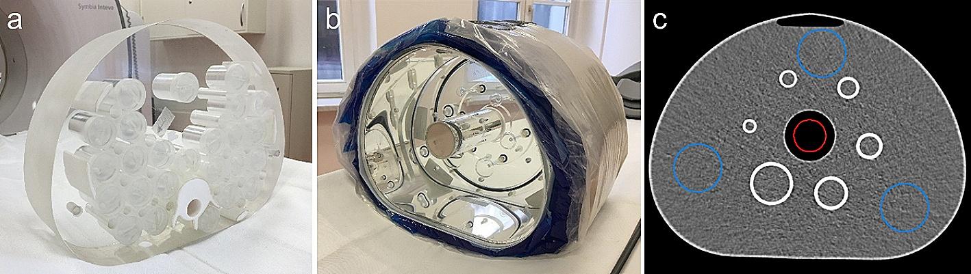
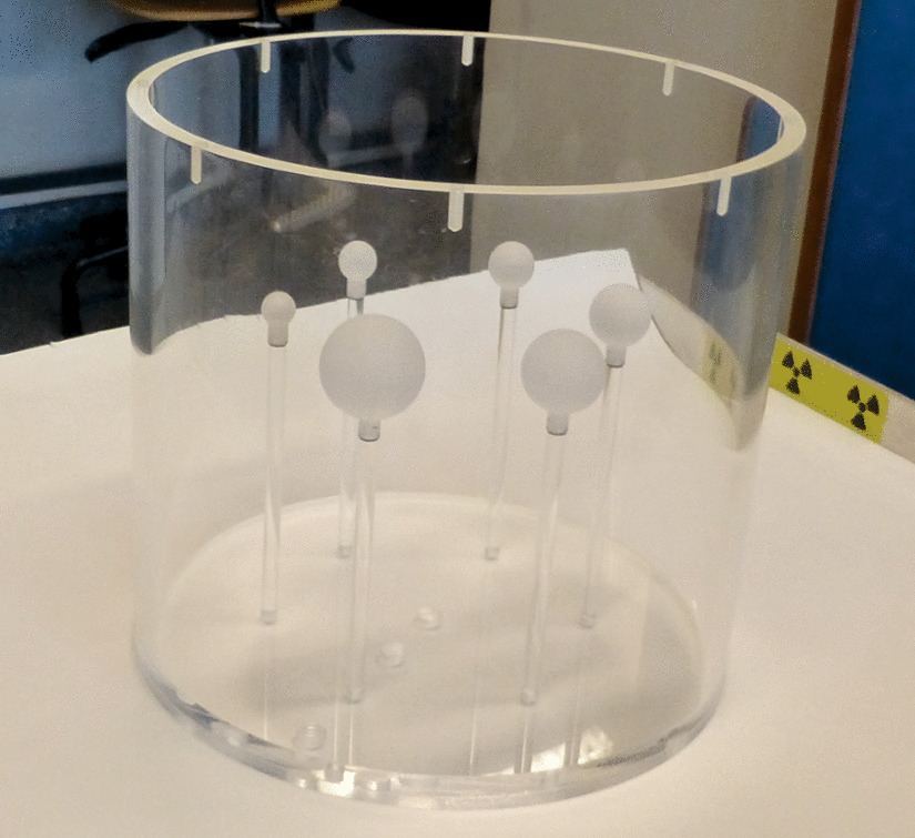
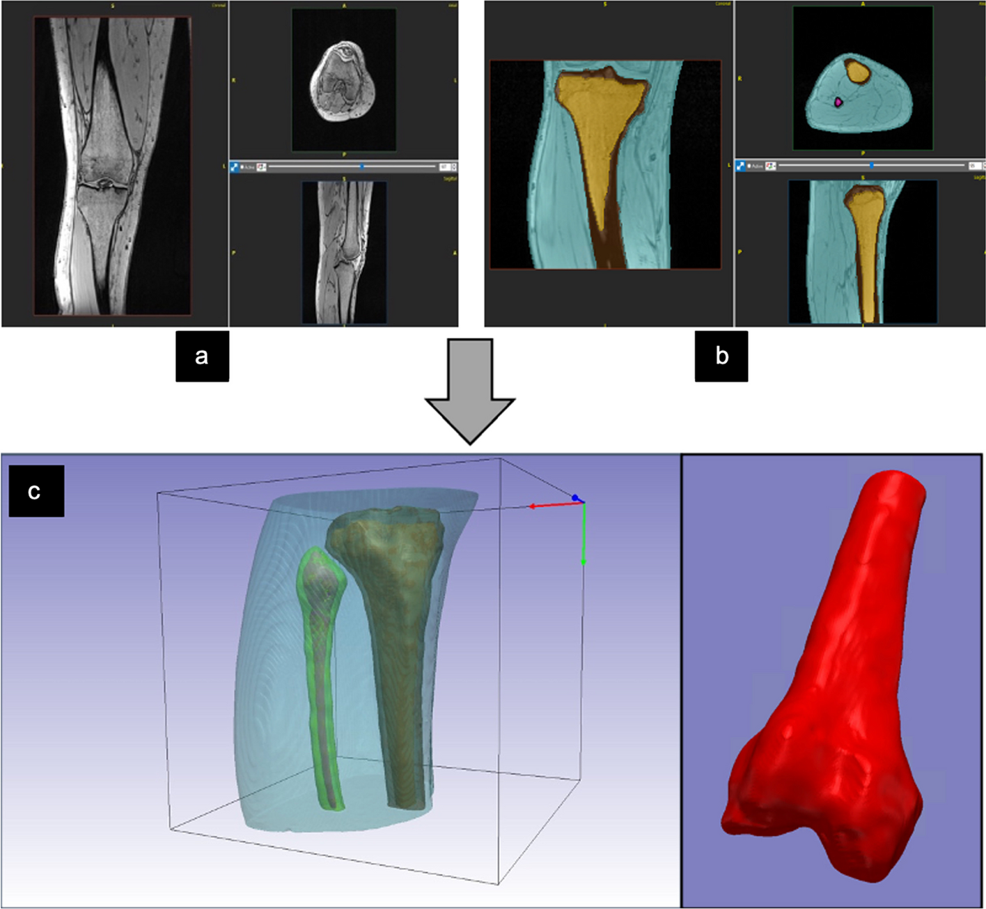
The SIM2 Bone Phantom (Kyoto Kagaku, Kyoto, Japan) [15, 21] was used. This phantom can reproduce tumor bone area in the vertebral body with four different diameters (13, 17, 22, and 28 mm) using the whole vertebral body as reference (diameter and length of 36 mm and 35 mm, respectively) (Fig. 1). The 99mTc activity concentrations of the normal vertebras, tumor, and mediastinum of the phantom filled with 99mTc were 50, 300, and 8 kBq/mL, respectively [15]. The lung insert was not filled with radioactive material.

Overview of the SIM2 phantom and enclosed radioactivity concentration

Phantom SPECT/CT images were acquired using Discovery NM/CT 860 (GE Healthcare) with a LEHRS collimator. For the dual-energy window scatter correction (SC) method (scatter weighting factor k was 1.10), the primary and scatter window acquisitions were 140 keV ± 10% and 120 keV ± 5%, respectively. The matrix size for the acquisition was 128 × 128, the magnification ratio was 1.0, the pixel size was 4.42 mm, and the projection number was 60 (step of 6°); automatic proximity was used, and the images were acquired with SwiftScan and SSM. The acquisition time was 6, 10, 30, and 60 s/view for SSM. In SwiftScan SPECT, counts are also acquired during 6° step detector rotation; 0–3°counts were added to the previous position view and 3–6°counts were integrated into the next position view. Thus, acquisition time per projection for SwiftScan was added to the detector rotation time (approximately 4 s per view) to that of SSM. Here, the scan time was defined as the start of projection data acquisition to its end. The scan times for SwiftScan SPECT and SSM were 5 min 4 s, 7 min 4 s, 17 min 4 s, and 32 min 4 s. The scans were performed in increasing order of scan times, and the counts and quantification values obtained were decay-corrected by the elapsed time from the start time of the first scan. CT images for attenuation correction (AC) were acquired at 120 kV and 30 mA with a 512 × 512 matrix, 1.675 pitch, and 1.0 s rotation and reconstructed at a 1.25 mm slice thickness with adaptive statistical iterative reconstruction (SS80 Slice 80%). All acquired projection images were reconstructed using a three-dimensional iterative ordered subset expectation maximization algorithm considering the CT-based AC, dual-energy SC, and resolution correction (Evolution for bone, GE Healthcare) without a noise reduction filter. The various combinations of the number of subsets and iterations were 10 (fixed) and 1–10, respectively. After reconstruction, a quantitative analysis software (Q.Volumetrix, GE Healthcare) was used to automatically resample both the CT and SPECT images to a voxel size of 2.21 × 2.21 × 2.21 mm3 prior to setting the volume of interest (VOI). This software calculates quantitative values using the planar sensitivity-based calibration method [13, 22, 23]. In this study, the Q.Volumetrix used was designed to calculate quantitative values without noise reduction filters. Therefore, all SPECT image quality evaluations were performed using SPECT images without noise reduction filters.

The system planar sensitivity was measured using the automatic mode provided by the manufacturer (GE Healthcare). A plastic petri dish with 99mTc solution (124.4 MBq) was placed on styrene foam (10 cm thickness) at the collimator surface, and the image was acquired from the anterior and posterior views. The primary and scatter window acquisitions were 140 keV ± 10% and 120 keV ± 5%, respectively. The system planar sensitivity was calculated using the following formula:

$$}\left( }/}} \right) = \left( }} kC_}} } \right)/}$$

(1)

where A is the decay-corrected activity at the start time of acquisition, T is the acquisition time, k is the scatter weighting factor, and Cp and Cs are the averages of the total counts in the anterior and posterior images for the primary and scatter windows, respectively. The measured system planar sensitivity was 88.4 cps/MBq.

To determine the optimal number of iterations, the convergence of 5- and 32-min acquisition was assessed. Based on the CT images, sphere-shaped VOIs were drawn at the center of each tumor bone area (28-mm hot sphere). The sizes of the VOIs were 80% of that of each hot sphere. The measured maximum and mean radioactivity concentrations (MBq/mL) were obtained using Q.Volumetrix.

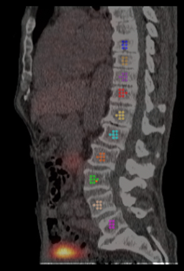
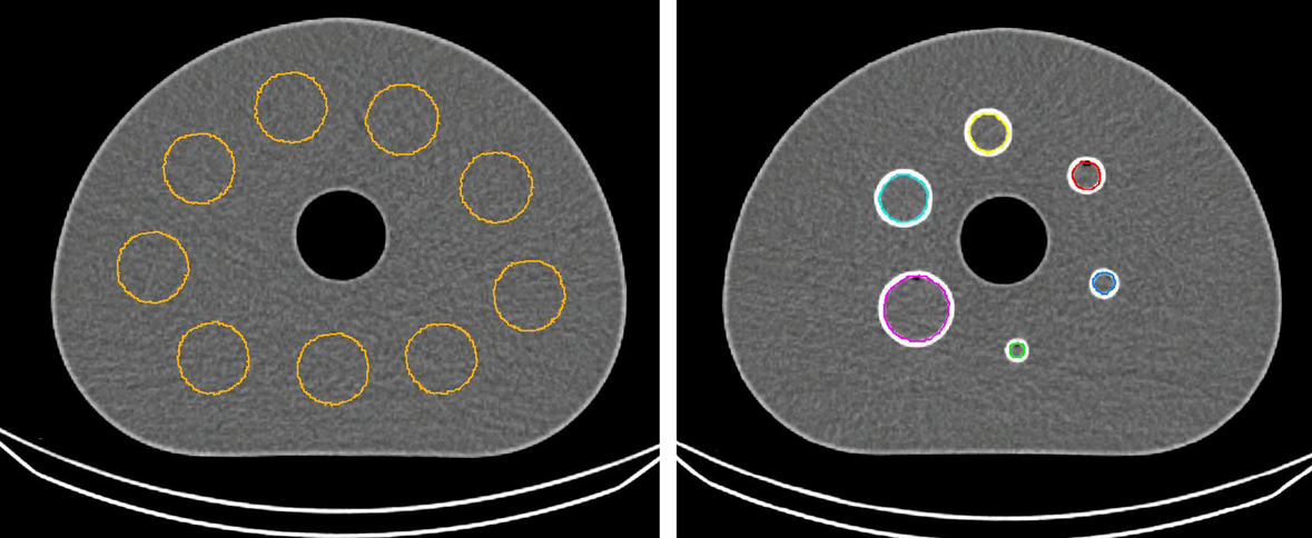
SPECT images obtained from each acquisition method were compared in terms of normal bone coefficient of variation (CV), contrast-to-noise ratio (CNR), full width at half maximum (FWHM), and quantitative value. For measuring image quality indices, a circular region of interest (ROI) with 80% of the diameter was set in five slices (Fig. 2), including the normal bone portion of the axial image. Similarly, ROIs were set in a slice with the largest diameter of the 17-mm-diameter tumor area. ROI settings were based on CT images. The mean count and standard deviation were obtained from the ROIs of tumor and normal areas. The CV was calculated using the following formula:

$$} = \frac}}} }}}}} }}$$

(2)

where Cnormal and CSD represent the mean count and standard deviation of the normal bone area, respectively.

Settings of the region of interest for evaluating image qualities

The CNR was calculated using the following formula:

$$} = \frac}}} - C_}}} }}}}} }}$$

(3)

where Ctumor is the mean count of the tumor area.

The effect of scan time on the count statistics of the tumor bone areas was investigated under the optimum number of iterations. Further, the spinous process line profile curves were obtained from five slices of the phantom (Fig. 2), and the FWHM was averaged from those slices using the Prominence processor version 3.1 software [23]

Based on the CT images, sphere-shaped VOIs were drawn at the center of each tumor bone area (13-, 17-, 22-, 28-, and 36-mm hot spheres). The sizes of the VOIs were 80% of that of each hot sphere. The measured mean radioactivity concentration (MBq/mL) was obtained using Q.Volumetrix. The error between the true and measured radioactivity concentrations at each tumor bone area was calculated using the following formula.

$$}\left( \% \right) = \frac}}} A_}}} } \right) }}}}} }} \times 100$$

(4)

where ATrue represents the radioactivity concentration in the tumor bone area of the phantom and ASPECT represents the mean radioactivity concentration in the tumor bone area obtained from the SPECT image. Here, ATrue was 300 kBq/mL.

In addition, to evaluate overall quantitative accuracy, the mean absolute error (MAE) of the measured radioactivity concentration for each examination time of SSM and SwiftScan SPECT was calculated.

$$} = \frac\mathop \sum \limits_^}} \left| }}} - A_}}} } \right|$$

(5)

where n represents the number of tumor bone regions and Ai,SPECT represents measured mean radioactivity concentration in tumor bone sphere size of i mm.