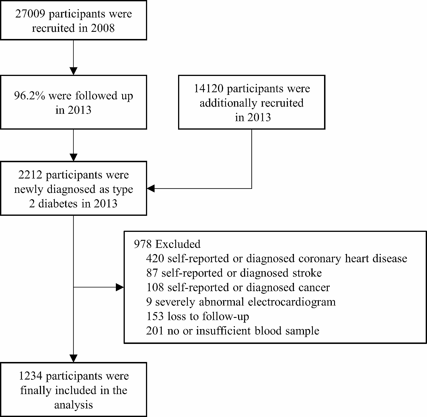
The NHANES is a cross-sectional nationwide survey to assess health and nutritional status of the noninstitutionalized U.S. population [19]. The current study was based on the NHANES 2007 to 2010 samples, because different information was collected in each survey cycle, and these were the most recent cycles that had released the variables of interest. Analyses for this study were limited to adults aged 20 years and older, which the NHANES had set as the age restriction for participants to receive adult-specific questionnaires. After excluding participants with missing information on variables of interest (i.e., serum PLP concentration and potential predictors), n = 3778 participants were included in the current study (Supplemental Fig. 1). NHANES was approved by the Institutional Review Board of the National Center for Health Statistics. Informed consent was obtained from all participants.

Serum vitamin B6, in the form of PLP, was measured by investigators at NHANES using reversed-phase high-performance liquid chromatographic (HPLC) with fluorometric detection at 325 nm excitation and 425 nm emission. Because chlorite post-column derivatization could oxidize PLP to a more fluorescent carboxylic acid form, post-column introduction of a sodium chlorite derivatization reagent was incorporated into the HPLC system to improve the PLP signal [20]. Quantification was based on analyte peak area interpolated against a five-point calibration curve obtained from aqueous standards. The mean coefficient of variation for the assay was 4.9% and the detection limit of the assay was 0.3 nmol/L [21].

Information on dietary intake was obtained using two 24-h dietary recall interviews. The first 24-h recall interview was conducted in-person in the NHANES Mobile Examination Center (MEC) at the same timepoint with examination components and biospecimen collection, and the second day was collected by telephone 3 to 10 days later. Two well-trained dietary interviewers administered the dietary interview at each MEC comprising three sections: (a) dietary recall, (b) nutritional supplement and antacid use, and (c) post-recall [22]. Average dietary intake, based on the 2 days, were used in the current analysis. The U.S. National Center for Health Statistics was responsible for the sample design and data collection and U.S. Department of Agriculture (USDA) Food Surveys Research Group was responsible for the dietary data collection methodology, maintenance of the databases used to code and process the data, and data review and processing [23]. The foods and beverages in the dietary interview components were converted to the 37 USDA food groups (Supplemental Table 1), based on the Food Patterns Equivalents Database (FPED). The FPED served as a unique research tool to evaluate foods and beverage intakes of Americans with respect to the 2015-2020 Dietary Guidelines for Americans [24].

Information on dietary supplement use was collected after the 24-h dietary recall for foods and beverages, using a similar protocol. Information was obtained on all vitamins, minerals, herbals, and other dietary supplements as well as non-prescription antacids that were consumed during a 24-h time period (midnight to midnight), including the name and the amount of supplement taken. Daily vitamin B6 supplement intake was calculated using the NHANES Dietary Supplement Database [25].

Demographic variables (age, sex, race/ethnicity, education level, and the ratio of family income to poverty), lifestyle factors (smoking status and physical activity), and information on medication use were derived from questionnaires in the home by trained interviewers, using the Computer-Assisted Personal Interviewing system. Education level was the highest grade completed by the participant, and was described as < 12 years (middle and elementary school), 12 years (high school) and > 12 years (college and graduate School). The income-to-poverty ratio reflected the ratio of an individual’s household income to the federal poverty level, adjusted for household size and composition [26]. Smoking status was categorized as never, former, or current smoking. Physical activity was categorized as below (< 150 minutes per week of moderate-intensity), meeting (150-299 minutes per week of moderate-intensity), or exceeding (≥300 min per week of moderate-intensity) the federal physical activity guideline recommendations [27]. Medication use included antihypertensive, antiglycemic, cholesterol-lowering agents and use of insulin (Yes/No for each). Systolic and diastolic blood pressures were measured three times from the seated position. If a blood pressure measurement was interrupted or incomplete, a fourth attempt was made [28]. The average of all available readings was used for analysis. Body mass index (BMI) was calculated as body weight (kg) divided by the square of height (m2). Blood triglycerides, high-density lipoprotein cholesterol (HDL-C), low-density lipoprotein cholesterol (LDL-C), and fasting plasma glucose were measured using a Roche Modular P chemistry analyzer. Glycosylated hemoglobin was measured on an A1c G7 HPLC Glycohemoglobin Analyzer (Tosoh Medics, Inc., 347 Oyster Pt. Blvd., Suite 201, So. San Francisco, Ca 94,080.). C-reactive protein assays were performed on a Behring Nephelometer [29].

Statistical analyses and all the computations for the current study were conducted with SAS 9.4 (SAS Institute Inc., Cary, NC) and Python 3.5 (Python Software Foundation, Delaware City, DE). The deep neural network structure was constructed with PyTorch (Adam Paszke, Sam Gross, Soumith Chintala, Gregory Chanan) [30]. PyTorch is an open source machine learning library for Python, used for applications such as computer vision and natural language processing. PyTorch has Graphical Processing Unit (GPU) support on tensor computation and an automatic gradients computing system [31].

Simple random sampling was used to divide the labeled dataset into training and test datasets with PROC SURVEYSELECT in SAS. The training set is a dataset of examples used for learning. By constructing a loss function based on the training set and finding a local (even global) minimum of the loss function, we can obtain good parameters or weights in the network to fit the training set. We assume that the test set followed the same probability distribution as the training set; if our model fits the training set, it also should fit the test set well. In general, there is no clear criterion for the ratio of training and test datasets. Samples are usually split, based on the data quality and sample size, with different ratios; the ratio of 90%:10% has been commonly used in previous studies [32, 33]. We held out 10% of the labeled dataset as the test dataset, which was used to determine the final model performance, and thus excluded from model development or tuning. In order to obtain a stable prediction model, we trained and selected a model using the remaining 90% as training data. Once the final model had been selected, we tested the performance on the 10% test sample, using R2 as the proportion of the variance in the dependent variable that was predictable from the independent variables. R2 is a function of the total sum of squares (SST) and the sum of squared errors (SSE) (\(^2=1-\frac\)). For both the DLA and MLR models, we developed two models: first, including food groups and vitamin B6 supplement intake and, second, including food groups, vitamin B6 supplement intake, and other aforementioned potential non-dietary predictors.

Deep neural networks are a class of models within the machine learning area which identify a nonlinear relationship between the input, x, and the output y [27]. Normally there are three types of layers in neural networks, the input layer, the output layer and the hidden layer (see Fig. 1 for an example). With an appropriate number of hidden layers, with certain nodes for each hidden layer, the neural network can be used to approximate the nonlinear function, y ≈ f(x). In our DLA model, we used a 4-hidden-layer fully connected neural network with the width of 30 nodes for each layer. Each neuron was connected by all the neurons in the previous layer (Fig. 1). In particular, the mathematical expression of the DLA model is following:

$$f\left(x;P\right)=_5\sigma \left(_4\sigma \left(_3\sigma \left(_2\sigma \left(_1x+_1\right)+_2\right)+_3\right)+_4\right)+_5,$$

where x is the input data, P is the parameter set, namely, P = , i = 1, ⋯5, and σ(x) is the rectified linear unit (ReLU) activation function [34] which has the form of the following form:

$$\upsigma \left(\mathrm\right)=\max \left(x,0\right)$$

The structure of neural network

Theoretically speaking, this neural network setup can approximate any dependencies between the input and the output, when the number of layers and nodes is large enough [35]. In particular, when the data have nonlinear dependencies, neural networks are able to perform better than regression, which is designed to reconstruct only linear dependencies and to ignore the nonlinearities. Moreover, regression models can be recovered by a simple neural network which only involves the input and output layers but no hidden layers.

To find the optimal parameter set, we needed to solve an optimization problem to minimize the distance between the empirical data and the model prediction, namely,

$$\undersetL(P)\triangleq \frac\sum_^n_i,P\right)-_i\right|}^2,$$

which is the loss function in machine learning. Here includes the training data and labels, and n is the number of participants in the training set. To solve this optimization problem, we employed the Adam algorithm [36], an algorithm for first-order gradient-based optimization of stochastic objective functions, based on adaptive estimates of lower-order moments, as our optimization method. We chose 0.001 as the learning rate to prevent overshooting which means wandering around the lowest point, because the learning rate was too high for the model when applying a gradient-based optimization algorithm. To prevent overfitting, we used batch normalization [25] and dropout [37], with a probability of 0.5, as regularization—a method to prevent overfitting by adding the norm of weight parameters to the loss function.

Because we were only interested in the description of samples without making any inferential conclusion in this study, we developed two MLR prediction models using the training data, including dietary and non-dietary predictors, as detailed above. To compare with the DLA models, we did not exclude any potential predictors in the MLR model based on their significant levels.

To test the robustness of our results, we conducted two sensitivity analyses. Because vitamin B6 supplement intake was strongly correlated with serum PLP concentration, we conducted subgroup analysis, stratified by vitamin B6 supplement use status (yes/no). We then included only variables identified by a stepwise regression model of the MLR (p = 0.5 for entry, and p = 0.1 for removal) in the DLA prediction model. Stepwise regression is a modification of the forward selection and backward elimination technique. As in the forward selection technique, variables are added one at a time to the model, as long as the F statistic p-value is below the specified α. After a variable is added, however, the stepwise technique evaluates all of the variables already included in the model and removes any variable that has an insignificant F statistic p-value exceeding the specified α. Only after this check is made and the identified variables have been removed can another variable be added to the model. The stepwise process ends when none of the variables excluded from the model has an F statistic significant at the specified α and every variable included in the model is significant at the specified α.