1 INTRODUCTION

Mobile EEG (electroencephalography) is becoming increasingly popular in cognitive neuroscience. This is because it allows us to begin studying brain activity in circumstances outside of typical controlled laboratory settings. These ambulatory experiments may be better able to describe the way the brain works in real life. However, movement can cause noise, which in turn can lead to negative effects on EEG signal quality and statistical power (Boudewyn et al., 2018; Luck, 2014). It is, therefore, important to find solutions that facilitate good signal quality in mobile EEG acquisition.

Here we define noise as sources of variation in the collected data that are unrelated to the event-related potential (ERP) components measured (Luck, 2014). Non-neural noise, from both physiological and environmental sources, can have a large influence on the statistical power of EEG and ERP recordings (Boudewyn et al., 2018; Luck, 2014). Physiological noise includes muscle activity, eye blinks, and movements, skin potentials, and cardiovascular activity (Gratton et al., 1983; Jung et al., 2000; Kappenman & Luck, 2010; Keil et al., 2014; Mathewson et al., 2017). Another source of EEG data noise is mechanical noise, which refers to artifacts that occur due to movement or locomotion, such as wire movements (Gwin et al., 2010; Symeonidou et al., 2018). The latter two types of noise are typically dealt with by restricting movements, and when this is not possible, advanced signal processing methods may be required. However, it is also possible that some particular EEG electrode features are more suitable for dealing with noise caused by mobile recordings than others.

Previous studies of electrode types tend to focus on the comparison between the use of active and passive signal transmission or amplification. Active-transmission electrodes use a small circuit board mounted on the electrode to pre-amplify signals directly on the surface of the scalp (i.e. pre-amplification) before passing these signals on to the amplifier (i.e. amplification), while passive electrodes simply collect the signals at the scalp which are then transmitted to the amplifier. Throughout this paper, we will use the terms “active” and “passive” to refer to whether signals were amplified at the scalp and amplifier (i.e. active-transmission) or only at the amplifier (i.e., passive-transmission), respectively. This pre-amplifier amplification at the scalp in active electrode configurations may help to achieve good signal quality by reducing detrimental effects of high impedance (Laszlo et al., 2014) and wire movements (Xu et al., 2017) on the data. Mobile passive electrode systems typically use a configuration with short wires that are fixed to the head and/or bundled together, as well as a small amplifier mounted directly on the head, in order to avoid the effects of wire movements (De Vos, Gandras, et al., 2014; De Vos, Kroesen, et al., 2014; Debener et al., 2012). While both of these configurations have been shown to collect laboratory quality EEG data during movement (De Vos, Gandras, et al., 2014; De Vos, Kroesen, et al., 2014; Debener et al., 2012; Scanlon et al., 2019, 2020) they have yet to be compared systematically using the same amplifier.

Laszlo et al. (2014) investigated differences between active and passive electrodes by having participants perform an auditory oddball task either with high or low impedance levels. They found that at low levels of electrode impedance (<2 k ) passive electrodes had better signal quality, with significantly lower levels of root-mean-squared (RMS) data noise. However, at higher impedance levels, active-transmission electrodes performed better, suggesting that, when application time is critical, active-transmission electrodes may be a good choice. A similar study by Mathewson et al. (2017) compared passive wet (with gel), active wet (with gel), and active dry (without gel) electrodes using the same amplifier. Active dry electrodes showed increased RMS data noise and lower statistical power. Moreover, active and passive wet electrodes showed similar levels of data noise, with passive electrodes performing better at single-trial RMS data noise, and active wet electrodes having lower ERP data noise. These studies show some interesting differences between active and passive electrode systems, but they did not address the issue of movement during data recording.

Oliveira et al. (2016a, 2016b) had participants perform an auditory oddball task, while both sitting and walking on a treadmill, with three different electrode configurations: Biosemi wet (Active), Cognionics wet (Passive with active shielding), and Cognionics dry (Passive with active shielding). The wet systems outperformed the dry system, with the active system showing almost no statistical differences between the seated and walking conditions for all metrics, including prestimulus data noise, and signal-to-noise ratio (SNR). The wet systems also showed high test-retest reliability for prestimulus data noise during both conditions, but only the active-wet electrode system demonstrated high test-retest reliability in the SNR and P3 time window amplitude variance. However, this study used different amplifiers and electrode set-ups when comparing the active and passive electrode systems, and therefore it is not known whether electrode differences, amplifier differences or electrode set-up accounted for the observed results. Nathan and Contreras-Vidal, (2016) demonstrated negligible motion artifacts with active electrodes during a walking task at speeds up to 3 km/hr, with some evidence of motion artifacts at 4.5 km/hr. De Vos, Gandras, et al. (2014) and De Vos, Kroesen, et al. (2014) found no significant difference in single-trial data noise between sitting and walking during an oddball task, while using a passive electrode system and a head-mounted amplifier. Other studies have compared wet and dry electrode types, among which some of them (e.g. Kam et al., 2019; Marini et al., 2019; Mathewson et al., 2017) found that dry electrodes capture valid EEG signals. However, we are not aware of any reports evaluating the performance of dry electrodes during natural behavior (e.g., walking), other than Oliveira et al. (2016a, 2016b). Additionally, dual-electrodes consisting of an additional layer of mechanically coupled and inverted secondary electrodes which record only electrical noise and motion artifacts have also been used to effectively collect EEG data during mobile tasks (Nordin et al., 2018, 2019a, 2019b, 2019c). As of yet, there has not been a comparison study of active and passive electrode configurations during a mobile task using the same mobile EEG amplifier.

A task commonly used in studies evaluating mobile EEG systems is the auditory oddball task. Rare, task-relevant auditory events typically generate a P3 component, a positive deflection recorded approximately 250–500 milliseconds following a rare stimulus to which one has been asked to attend (Luck, 2014). The P3 component has been extensively studied, and can be observed reliably with low trial numbers, even at the single-trial level (e.g. De Vos, Gandras, et al., 2014; De Vos, Kroesen, et al., 2014). The oddball task can also be used in a dual-task scenario to infer changes in attention, as attention to a primary task typically reduces the P3 amplitude to salient events in the secondary, oddball task (Polich, 1987; Polich & Kok, 1995). In previous mobile EEG studies, the auditory P3 component has been shown to decrease in amplitude by up to 30% during mobile dual-tasks such as walking (De Vos, Gandras, et al., 2014; De Vos, Kroesen, et al., 2014; Debener et al., 2012; Ladouce et al., 2019), cycling (Scanlon et al., 2019, 2020; Zink et al., 2016), and simulated driving (Chan et al., 2016) compared to the stationary oddball task. This has been interpreted in previous research to be because the mobile task takes attentional resources away from the oddball task, however research with animal models has suggested that this may be due to the inhibition of the auditory cortex by motion and motor system activation (Nelson et al., 2013; Nordin et al., 2019a, 2019b, 2019c; Otazu et al., 2009; Schneider et al., 2014). Interestingly, Ladouce et al. (2019) showed that simply being wheeled around without intentional movement was enough to significantly reduce the P3. The P3 has also been shown to be somewhat unique to individuals, as several studies have demonstrated test-retest reliability in P3 amplitude for different conditions (De Vos, Gandras, et al., 2014; De Vos, Kroesen, et al., 2014; Debener et al., 2012). The P3 reduction effect appears to be very robust, despite several of these studies using different EEG systems and demonstrating increases in measures of data noise such as SNR and data noise during walking (Debener et al., 2012) and biking (Scanlon et al., 2019; Zink et al., 2016).

The current study built on the body of mobile EEG and electrode comparison literature, and aimed to further understand how to best record EEG experiments in real-world circumstances. For mobile EEG studies, both active and passive electrodes require specific configurations according to their capabilities, and most EEG manufacturers do not have any system available that works identically with both active and passive electrodes. Therefore, this study reflects not only amplification style, but rather a comparison of the typical mobile active electrode configuration versus the typical mobile passive electrode configuration. Specifically, we aimed to learn whether there is a benefit to having pre-amplification that takes place on the head followed by amplification in a backpack (i.e. active electrode configuration), compared to a system using the same mobile amplifier, with highly restricted short wires and amplification only on the head (i.e. passive electrode configuration). In this experiment, participants performed two 6-min blocks of an auditory oddball task, while both standing and walking outdoors. ERP magnitude, morphology, and topography for the P3 were analyzed, as well as measures of prestimulus ERP data noise and SNR. In one session a passive electrode configuration was used, and in another session, an active electrode configuration was used. Before exploring our main hypotheses, we intended to validate our measures by confirming that participants did not have significantly different cadences between walking conditions, and also showed significant differences in P3 amplitude between standards and targets in the oddball task. Our first hypothesis was that similar to previous studies, P3 amplitude would decrease during walking for both electrode types. The second hypothesis predicted that measures of data quality (i.e. post-trial rejection trial numbers, pre and post-trial rejection SNR and data noise) would also decrease due to increased noise in the walking condition. The third hypothesis predicted that an active electrode configuration would perform better in measures of post-trial rejection trial numbers, data noise, and SNR (both pre and post-trial rejection) than passive electrodes during movement. Finally, as our task involved collecting data from participants during standing and walking on two separate days, this offered the opportunity to quantify the test-retest reliability of P3 amplitudes and measures of data quality.

2 METHODS 2.1 Participants

Twenty-six individuals participated in the study, recruited through the Oldenburg University website. Data from seven participants were removed from the study due to technical issues during data collection. This was mainly due to problems in the wireless connection, which have since been addressed with the manufacturer and solved. Data from one participant were removed due to scheduling issues for the second appointment. This left 18 participants (mean age = 24; age range: 20–28; eight female) for the final analysis. Participants had no history of psychiatric or neurological problems and received an honorarium of 10 €/hour. Experimental procedures were approved by the Oldenburg University ethics committee.

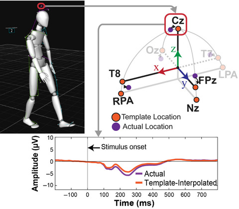
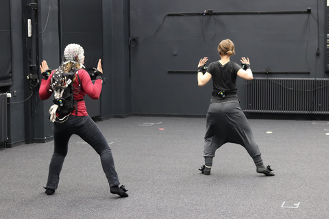
2.2 Materials

All participants came in for two separate recording sessions, approximately 3–15 (Mean (M) = 6) days apart, to record with each electrode type. Electrode type order was counterbalanced across participants. Recording time of day was within the same hour for 10 participants, and earlier/later times were counterbalanced according to electrode type in cases where the same time could not be scheduled for both sessions. For each experiment session, participants were fitted with an EEG cap with either active (actiCAP, EasyCap GmbH, Brain Products GmbH) or passive electrodes (EasyCap GmbH, Brain Products GmbH), each with identical 64 electrode layouts. Ground and reference electrodes were embedded at the AFz and FCz (10–20 system) locations in the cap, respectively. The same two Brain Products LiveAmp amplifiers, which consisted of one amplifier for channels 1–32 and one for channels 33–64 (which were never switched), were used for all sessions. A Faros 180° eMotion (Mega Electronics, 2017) accelerometer sensor was fixed to the right foot of each participant using elastic tape. The auditory oddball task was presented using NBS (Neurobehavioral Systems) Presentation on a Dell (Latitude 5289) Ultrabook and earphones (Sony MDR-E9LP). Data were collected using the same Ultrabook, using LSL (Lab Streaming Layer) software to time-synchronously collect both the EEG channel data and the event markers from NBS Presentation. During active electrode sessions, the LiveAmp and Ultrabook were placed into a small backpack that was customized for the ventilation of the computer. All loose wires were tucked into the backpack to minimize wire movements. During passive electrode sessions, the LiveAmp was fixed to the top of the participant's head using elastic tape and a customized sponge that included holes to avoid any direct physical pressure on underlying electrodes (Figure 1a). The Ultrabook was also placed in the backpack for passive electrode sessions. At the beginning (and end) of each session, synchronization reference signals were sent into EEG and accelerometer data. To do this, the LiveAmp and Faros sensors were plugged into a sync-box after recordings were started and before they were stopped. Custom MATLAB scripts were used to offline prune the data streams into one synchronized data file. The experiment took place in an outdoor (roofed) basketball arena at the Oldenburg University campus. Pylons were placed in a rectangular formation around the whole arena and occasionally adjusted to avoid rain or excessive sunlight.

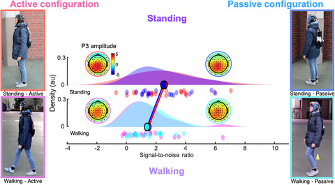
Conditions and pre-processing. (a): The four conditions used during the oddball task (staged image): Standing with active electrodes (top left), standing with passive electrodes (top right), walking with active electrodes (bottom left), walking with passive electrodes (bottom right). (b) Preprocessing pipeline used for all conditions

2.3 Experiment set-up

Participants were asked to wash and dry their hair prior to the beginning of setup. During the EEG setup, gel was used to bridge the gap between the electrodes and the scalp. For active electrodes, SuperVisc High-Viscosity Electrolyte-Gel was used (according to Brain Products GmbH recommendations), and a blunt-tip syringe was used to mildly abrade the skin and move hair in order to adjust the impedance and connection. For passive electrodes, preparation started with alcohol applied using a cue tip, followed by the application of Abralyt HiCL Abrasive Electrolyte-Gel, also adjusted for impedance using a cue tip. Impedances were adjusted using Brain Vision Recorder software, with signals wirelessly sent from the LiveAmp to the Ultrabook. Impedance was adjusted to <10 kΩ for each electrode. After preparation, all the needed equipment was moved to the outdoor arena for data recording. The experimenter then adjusted the audio volume to the participant's comfort level and began the recording.

2.4 Experiment task and procedure

The whole experiment included three separate tasks; however, only one is described in the current study. Participants performed an auditory oddball task using headphones, while both standing next to a wall and walking around the arena (Figure 1a). In a third condition, participants walked with an experimenter; however, this will be described in a separate paper. During the standing condition, participants stood with their eyes open, staring at a brick wall. During the walking condition, participants walked at their own pace around the arena in a clockwise direction, following pylons as a guide. They were encouraged to keep a leisurely, slow pace in order to avoid aerobic effects.

Each condition block included an oddball task, in which participants were asked to silently count the number of deviant (target) tones. This included a set of 280 trials (15% deviants) plus 1–30 extra trials in order to keep the number of deviants unpredictable. Trial numbers before preprocessing were approximately equivalent between conditions (Standing Active: Mtarg = 77.33, Standard deviationtarg (SD) = 3.68; Mstand = 508.22, SDstand = 13.07; Standing Passive: Mtarg = 77.94, SDtarg = 3.84; Mstand = 510.06, SDstand = 16.33; Walking Active: Mtarg = 79.17, SDtarg = 3.29; Mstand = 514.83, SDstand = 10.74; Walking Passive: Mtarg = 78, SDtarg = 3.58; Mstand = 514.11, SDstand = 12.78). Additionally, the task was set to avoid playing two deviants subsequently. The tones were 800 and 1,000 Hz, and their standard (frequent) or target status was counterbalanced across participants. The inter-trial interval varied randomly between 500 and 1,500 ms (125 ms uniform distribution). This high variability was used in order to avoid a rhythm with which participants could synchronize their steps. Each block lasted approximately 5–6 min and was repeated twice for each condition, and counterbalanced. Participants reported the number of target tones counted to the experimenter at the end of each condition block.

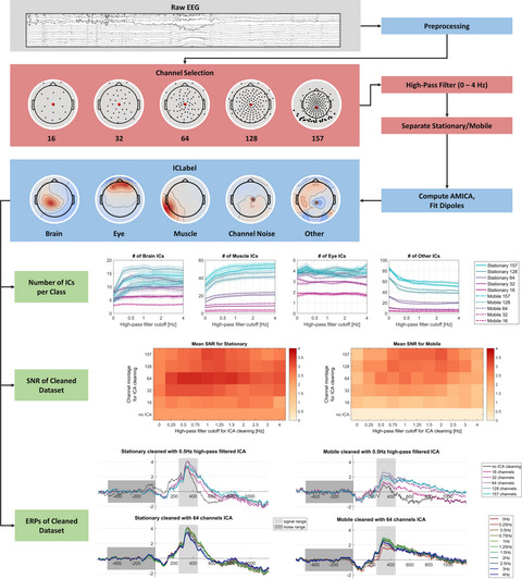
2.5 EEG preprocessing

Following data collection, EEG and accelerometer data were processed using EEGLAB 14.1.2b (Delorme & Makeig, 2004) and custom MATLAB scripts (Figure 1b). First, data from the accelerometer and EEG were synchronized using TTL pulses from the sync-box. The data were filtered with a high-pass filter (HPF; order 1650) of 1 Hz and low-pass filter (LPF; order 166) of 40 Hz, then resampled to 250 Hz. All filters were Hamming windowed, zero-phase finite impulse response (FIR) filters with a transition bandwidth at 25% of the lower passband edge (using EEGLAB function pop_eegfiltnew). Then, bad channels were removed using the function clean_rawdata (an EEGLAB wrapper function calling clean_artifacts), removing channels if they had a >5-s flatline, and <0.5 correlation to a reconstruction of the channel based on other channels. These parameters were kept conservative in order to remove objective outliers and allow noise caused during the data collection to be processed and later analyzed. One channel was removed from two active (electrodes TP10, P5) and three passive (electrodes PO8, PO10, Fz) datasets across all subjects. Following this, data were epoched into consecutive 1-s segments, and epochs with artifacts (channel and global thresholds of 2 standard deviations) were removed. Extended infomax independent component analysis (ICA) as implemented in EEGLAB was then run on the remaining concatenated 1-s epochs and ICLabel (Pion-Tonachini et al., 2019; see labeling.ucsd.edu) was used to identify and remove any components with over 85% probability of being eye-related or 40% probability of being due to heart activity (e.g. Viola et al., 2009). Then, all non-artifactual components were back-projected into continuous datasets, which were filtered with an HPF of 0.3 Hz (order 5500), and filtered again with an LPF of 40 Hz (order 166). The removed bad channels were then interpolated, and data were re-referenced to an average of TP9 and TP10. Data were then epoched to oddball events, beginning with the baseline 200 ms before the tone (at 0 ms) and ending 800 ms after the tone, creating 1-s epochs with 250 timepoints. Data were then baseline corrected from −200 to 0 ms. Segments with remaining artifacts were removed, this time with channel and global thresholds of 3 standard deviations.

2.6 Accelerometer preprocessing

Data collected from the right foot of each participant were used to determine cadence during the experiment. Right foot acceleration data (in mg's) were detrended and filtered with a low-pass filter of 30 Hz (2nd order Butterworth). A step detection algorithm was then used to mark step timing.

2.7 Prestimulus data noise and SNR calculations

Prestimulus ERP data noise was calculated by first averaging data from the Pz electrode over all artifact-removed trials, then taking the standard deviation of all time-points in the −200 to 0 ms interval before the tone onset, similar to previous studies (De Vos, Gandras, et al., 2014; De Vos, Kroesen, et al., 2014; Scanlon et al., 2017, 2019).

Signal-to-noise ratio (SNR) was calculated by first creating two ERPs per subject and condition, one for the even-numbered and one for the odd-numbered trials, and then taking the mean (i.e. signal) and the absolute difference (i.e. noise) between both (see Debener et al., 2007; Finneran et al., 2019; Kelly et al., 2014; Kremláček et al., 2012; Schimmel, 1967; Wright et al., 2011). The SNR was then obtained as the signal divided by the noise within the P3 time window for each subject. This procedure allows for measuring signal and noise at the same latency. SNR was then compared as an average for each subject between conditions. We were also interested in the effect of increasing trial numbers both without and with the factor of time, for our electrode and mobility conditions. Therefore, we plotted the SNR with increasing trial numbers both with time ignored by taking 100 trial permutations for each increasing number of trials and chronologically over time. We then performed the analysis using the final SNR value for each subject in each condition. To keep equal trial numbers (within trial-rejection type) in each condition the SNR value was calculated at the minimum trial number (the number of trials for the subject with the fewest trials) in each condition.

2.8 Statistical analysis

Data were analyzed using MATLAB (2016) custom scripts and JASP software (JASP Team, 2020). Cadence was assessed using a paired t test between the walking conditions of each electrode type. The P3 time window used was 284–484 ms, which was calculated by taking 100 ms before and after the average P3 peak time point for each subject and condition. This same time window was used for the SNR analysis. P3 amplitudes were computed by taking the mean of the P3 time window over all target trials for each participant (Luck, 2005a, 2005b). These values were then analyzed using repeated-measures 2 × 2 × 2 analyses of variance (ANOVA) with factors being electrode system (active/passive), mobile condition (standing/walking), and stimulus (standard/target), in order to first validate that the oddball task was performed correctly. Trial numbers and prestimulus data noise were analyzed using 2 × 2 ANOVAs with factors being electrode type and mobile condition. Trial numbers, P3 amplitude, and SNR were analyzed using 2 × 2 ANOVAs with the same factors, but using the target trials only. SNR pre and post-trial rejection, without and with time, were analyzed using repeated-measures 2 × 2 × 2 ANOVAs with factors being electrode system (active/passive), mobile condition (standing/walking), and trial rejection (trial-rejected/non-trial rejected). Effect sizes for p < .10 ANOVA effects were calculated using the partial eta squared (ηp2). As a post hoc test of the null hypothesis for signal quality, Bayesian repeated-measures ANOVAs were carried out on the P3 amplitude, prestimulus data noise, and SNR. This analysis allows for the interpretation of evidence for or against the null hypothesis; therefore, offering us further information about whether the electrode types are effectively the same according to our measures. ANOVA tests were followed up with Holm-Bonferroni corrected (Abdi, 2010; Holm, 1979) paired t tests, only for results with significant (or marginal) group effects addressing our main research questions. Effect sizes for p < .10 t tests were calculated using Cohen's d and 95% confidence intervals. Tests are considered significant at the level of ɑ = 0.05, unless otherwise stated, as in the case of Holm-Bonferroni corrected multiple t tests. Test-retest reliabilities were performed using an average value for each subject in each condition and were calculated as parametric (Pearson) correlations between electrode types for prestimulus data noise, SNR, and P3 amplitudes. These tests were then followed up with Shepherd's pi correlations, as the Shepherd's pi measure provides adequate statistical power and protects against false positives due to outliers (Schwarzkopf et al., 2012). In the figures, distributions for prestimulus baseline noise and SNR were calculated using the rm_raincloud function (modified by the authors; https://github.com/RainCloudPlots/RainCloudPlots/tree/master/tutorial_matlab). Shepherd's pi plots using Mahalanobis distance contours were created using Scatter Outliers (modified by the authors; Schwarzkopf et al., 2012) from the Shepherd toolbox.

3 RESULTS 3.1 Cadence

In order to validate that participants did not change their walking patterns in any systematic way, while using different EEG systems, we applied a step detection algorithm on the accelerometer right foot data to determine cadence (steps/minute) during the walking conditions. We found no significant difference in cadence between walking during active (M = 42.65 steps/min) and passive (M = 44.20 steps/min; Mdiff = −1.55; SDdiff = 6.46; t(17) = −1.02; p = .32) electrode conditions.

3.2 P3 Amplitude

ERP waveforms and P3 topographies are plotted in Figure 2. The highlighted regions in the plots illustrate a significant positive potential to the target stimuli peaking at approximately 385 ms. Inset maps also indicate that this potential had a posterior-central topography, as can be expected for a P3 component (De Vos, Gandras, et al., 2014; De Vos, Kroesen, et al., 2014; Debener et al., 2012). We investigated P3 amplitude by first performing a 2 × 2 × 2 ANOVA with factors of electrode system (active/passive), mobility (standing/walking) and stimulus (standard/target). Significant main effects of stimulus (F(1,17) = 69.52; p < .001; ηp2 = 0.80) and mobility (F(1,17) = 7.32; p = .015; ηp2 = 0.30) were found, but no main effect of electrode system (F(1,17) = 0.089; p = .77). Additionally, an interaction effect was found between mobility and stimulus (F(1,17) = 6.58; p = .02; ηp2 = 0.28). Target stimuli were most important in determining cognitive differences between the two mobility conditions, and were also used for the SNR analysis; therefore, these differences were further analyzed through a 2 × 2 ANOVA using only the target trials. Here, we found again a significant main effect of mobility (F(1,17) = 7.72; p = .013; ηp2 = 0.31), due to larger amplitudes during the standing condition than the walking condition (Figure 2). There was no effect of electrode system (F(1,17) = 0.09; p = .77) or interaction (F(1,17) = 1.42; p = .25).

Event-related potential (ERP) waveforms. Grand-average ERPs for each condition, computed at electrode Pz for both standard (black) and target (color/shades) conditions. Shaded regions indicate standard error of the mean. The P3 time window (284–484 ms) is highlighted. Scalp topographies show the grand-average of the P3 time window for target trials

To further investigate the patterns of P3 amplitude for the factors of electrode type and mobility, we followed up these results with a Bayesian ANOVA, including within-subject factor condition, using the same factors (Table 1). Here we found moderate evidence for the main effect of mobility (IBF = 4.97), moderate evidence against the main effect of electrode system (IBF = 0.25), and evidence against the interaction (IBF = 0.47).

TABLE 1. 2 × 2 Bayesian repeated-measures ANOVA for P3 target amplitude (mobility: standing and walking; electrode: active and passive). “Models” column shows predictors included in each model. The “P(M)” column shows the prior model probability. The “P(M|data)” column shows the posterior model probability. The “BF M” column shows the posterior model odds, and the “BF 10” column shows the Bayes factors of all models compared to the null model. The “error %” column shows estimates of the numerical error in the computation of the Bayes factor. All models are compared to the null model and are sorted from highest Bayes factor to the lowest Bayesian repeated-measures ANOVA Model comparison Models P(M) P(M|data) BF M BF 10 Error % Null model (incl. subject) 0.20 0.12 0.56 1.00 Mobility 0.20 0.61 6.29 4.97 1.57 Mobility + electrode 0.20 0.16 0.76 1.30 2.52 Mobility + electrode + mobility × electrode 0.20 0.08 0.33 0.61 4.63 Electrode 0.20 0.03 0.13 0.25 0.91 Note All models include subject. 3.3 Trial numbers

Table 2 shows the number of standard and target trials remaining after trial rejection for each condition. Analyzing trial numbers allows us to estimate levels of data noise in each condition before trial rejection procedures (Oliveira et al., 2016a, 2016b). We calculated differences between trial numbers following trial rejection in repeated-measures 2 × 2 ANOVA, with factors being electrode type (active/passive), and mobility (standing/walking), with target and standard trials added together. There was no main effect of electrode system (F(1,17) = 0.34; p = .57), but a significant main effect for mobility (F(1,17) = 57.2; p = 7.77e-7; ηp2 = 0.77). This demonstrated that more trials were lost in the artifact rejection process during the walking (M = 451.14; range = 374–515) conditions than the standing (M = 528.56; range = 410–589) conditions. Additionally, there was no significant interaction effect between mobility and electrode type (F(1,17) = 1.43; p = .25).

TABLE 2. Trial numbers after artifact rejection Number of trials remaining after artifact rejection Condition Targets Standards Mean Range SD Mean Range SD Active standing 68.39 57–80 6.59 454.67 353–499 35.54 Passive standing 70.72 61–81 5.86 463.33 376–508 27.64 Active walking 60.44 50–71 5.80 391.89 330–433 26.99 Passive walking 58.11 45–71 6.71 391.83 328–444 28.68 3.4 Prestimulus ERP data noise

Figure 3 (top) shows a distribution of the prestimulus data noise for each subject in each condition. The plot demonstrates an increase in data noise during walking compared to standing, but little difference between the electrode types. We used a 2 × 2 ANOVA with factors of electrode system (active/passive), and mobility (standing/walking). Here we did not find a significant main effect of mobility (F(1,17) = 3.42; p = .082; ηp2 = 0.17), electrode (F(1,17) = 0.24; p = .63) or interaction (F(1,17) = 0.15; p = .70).

Data noise and signal-to-noise ratio (SNR) Distributions. Top: Distribution of ERP prestimulus data noise for each condition. Small dots under the distributions refer to single-subject values; larger dots refer to group means per condition. Density is scaled in arbitrary units and calculated using the MATLAB function ksdensity. Distribution here refers to the representation of how often each value on the x axis occurs within the data. Bottom: Distribution of signal-to-noise ratio for each condition

To further understand the patterns of prestimulus data noise for the factors of electrode type and mobility, we followed up these results with a Bayesian ANOVA, including within-subject factor condition, with the same factors (Table 3). The purpose of this second ANOVA was to investigate whether there was evidence in favor of the null hypothesis. Here we observed moderate evidence for the main effect of mobility (IBF = 3.24), but moderate evidence against the main effect of the electrode (IBF = 0.26) as well as against the interaction (IBF = 0.31).

TABLE 3. 2 × 2 Bayesian repeated-measures ANOVA for ERP prestimulus data noise (mobility: standing and walking; electrode: active and passive). “Models” column shows predictors included in each model. The “P(M)” column shows the prior model probability. The “P(M|data)” column shows the posterior model probability. The “BF M” column shows the posterior model odds, and the “BF 10” column shows the Bayes factors of all models compared to the null model. The “error %” column shows estimates of the numerical error in the computation of the Bayes factor. All models are compared to the null model and are sorted from highest Bayes factor to the lowest Bayesian repeated-measures ANOVA Model comparison Models P(M) P(M|data) BF M BF 10 Error % Null model (incl. subject) 0.20 0.18 0.85 1.00 Mobility 0.20 0.57 5.29 3.24 1.67 Mobility + electrode 0.20 0.16 0.76 0.91 8.44 Mobility + electrode + mobility × electrode 0.20 0.05 0.20 0.28 1.98 Electrode 0.20 0.05 0.19