
記住我

The default mode network (DMN, or just default network, DN) is a brain network that becomes engaged during neuroimaging experiments when individuals are “left to think to themselves undisturbed” (Andrews-Hanna, Reidler, Sepulcre, Poulin, & Buckner, 2010), that is, when people are not engaged in external interactions and their “minds wander” (Buckner, Andrews-Hanna, & Schacter, 2008). Such spontaneous, nonintentional thoughts can be positive, such as daydreaming about positive things, or negative, such as ruminating on emotionally distressing issues. While there is disagreement on how to define “mind-wandering” (Christoff et al., 2018; Christoff, Irving, Fox, Spreng, & Andrews-Hanna, 2016; Seli et al., 2018) there is general consensus (i) that spontaneous, nonintentional thoughts can be positive or negative, (ii) that many individuals spend a significant amount of their time mind-wandering, and (iii) that a significant portion (about 10–30%) of mind-wandering is associated with negative thoughts (Fox et al., 2018; Killingsworth & Gilbert, 2010). Importantly, mind-wandering with negative thought content is often associated with negative moods: mind-wandering with negative thoughts content can cause negative mood (Killingsworth & Gilbert, 2010; Poerio, Totterdell, & Miles, 2013; Ruby, Smallwood, Engen, & Singer, 2013) and negative mood can cause mind-wandering with negative thought content (Smallwood, Fitzgerald, Miles, & Phillips, 2009; Smallwood & O'Connor, 2011).
Surprisingly little is known about the neural basis of positive or negative spontaneous, nonintentional thoughts, and to the best of our knowledge only very few functional neuroimaging experiments modulated the valence of thoughts to specify DMN activity associated with positive or negative thoughts during mind-wandering. A study by Tusche, Smallwood, Bernhardt, and Singer (2014) used a task with either positive or negative self-referential attribution, and multivariate pattern analysis (MVPA) to identify voxels providing significant classification information for positive versus negative thoughts. Such voxels were found in the medial orbitofrontal cortex (mOFC, a part of the DMN). Notably, that classifier predicted the valence of thoughts during task-free rest periods acquired during a second fMRI experiment 1 week later. Another study (Gorgolewski et al., 2014) assessed self-generated thoughts during fMRI with a questionnaire. Activity in the fronto-median cortex (extending into the mOFC) was negatively correlated with the questionnaire-factor “positive thoughts.” A study by Taruffi, Pehrs, Skouras, and Koelsch (2017) used sad-sounding and joyful-sounding music to modulate the quality of thoughts during mind-wandering. Functional neuroimaging data showed regions with higher eigenvector centrality (i.e., regions with influential positions within brain networks) during sad-sounding than joyful-sounding music in the ventromedial prefrontal cortex (vmPFC) including medial orbitofrontal cortex, and the anterior portion of the posterior cingulate cortex (area 23c of the PCC). Both mOFC and area 23c are subregions of the anterior and posterior midline “hubs” of the DMN (Andrews-Hanna et al., 2010). Other studies support the notion that DMN activity modulates the valence of thoughts during mind-wandering. A study by Karapanagiotidis et al. (2020) used resting-state fMRI data and retrospective descriptions of the participants' experience during the scan. The authors reported that a state associated with more negative thoughts related to an individual's past, was associated with DMN activity. In a study by Letzen and Robinson (2017), individuals were asked to experience the emotions of positive (“happy”) and negative (“sad”) autobiographical memories. The authors observed that pre-defined midline DMN regions showed increased functional connectivity with ventral anterior cingulate cortex (vACC) and posterior insula during negative thoughts compared to baseline. Taken together, these studies suggest a role of anterior and posterior midline structures of the DMN (including mOFC and area 23c) in generating and driving thoughts with emotional valence during mind-wandering, and that these DMN structures show functional connectivity with other structures, such as vACC and posterior insula, as a function of the valence of self-generated thoughts.
To further investigate this issue, we developed an experimental paradigm in which spontaneous, nonintentional thoughts are stimulated and modulated with music. In two previous studies (Koelsch, Bashevkin, Kristensen, Tvedt, & Jentschke, 2019; Taruffi et al., 2017), we showed that music, in addition to influencing emotions and moods, also often elicits mind-wandering, and modulates the valence of thoughts during mind-wandering. In the study by Taruffi et al. (2017), thoughts emerging during joyful-sounding music were more positive than thoughts emerging during sad-sounding music. These results were replicated in a second study (Koelsch et al., 2019), in which heroic-sounding music led to more positive thought contents than sad-sounding music. However, the study by Taruffi et al. (2017) left a number of controversial questions open: First, the strength of mind-wandering was higher during sad than joyful music, possibly due to sad music being slower and thus attracting less attention than fast music. Thus, it is unclear whether increased eigenvector centrality observed in the mOFC and area 23c of the posterior cingulate cortex modulated the valence of thought contents, or reflected the strength of mind-wandering. Second, due to the lack of a neutral baseline condition, it was not possible to determine whether thought contents during sad music were actually negative, or just less positive than during joyful music. Nevertheless, that study (Taruffi et al., 2017) was an ideal basis for the formulation of directional hypotheses for our current study.
Here, we devised an experimental paradigm with two types of positive music stimuli (joyful and peaceful) and two types of negative music stimuli (sad and nervous) in a way that positive music had on average the same tempo as negative music (joyful and nervous music was faster than peaceful and sad music). The aim, thus, was to modulate the valence of thought contents while controlling for the tempo of the music (and thus for the strength of mind-wandering), in order to identify differences in DMN activity between positive and negative thought. Moreover, we included rest-blocks without music, to compare data of blocks with positive or negative music to a neutral baseline condition. Based on our previous studies (Koelsch et al., 2019; Taruffi et al., 2017) we hypothesized that music would evoke mind-wandering with more positive thoughts during positive music, and more negative thoughts during negative music (compared to a neutral baseline), and stronger network (eigenvector) centrality in the midline-core of the DMN during negative compared with positive music (and compared with a neutral baseline), specifically in the medial orbitofrontal cortex and area 23c of the posterior cingulate cortex (for an illustration of eigenvector centrality see Figure S1). Should our findings accord with our hypothesis, they would indicate a neural basis for the modulation of the valence of thoughts during mind-wandering.
2 METHODS 2.1 ParticipantsThirty three participants (18 women, age-range 20–31 years, mean = 23.1 years) were included in the fMRI data analysis. Exclusion criteria were hearing impairment (as assessed with a standard pure-tone audiometry), musical anhedonia (as assessed with the Barcelona Music Reward Questionnaire; Mas-Herrero, Marco-Pallares, Lorenzo-Seva, Zatorre, & Rodriguez-Fornells, 2013), and previously diagnosed neurological or psychiatric disorder (according to self-report). None of the participants were professional musicians, 11 participants had never played an instrument, nine participants played an instrument or sang, but without having received instrument or singing lessons, and nine participants had received instrumental or singing lessons for an average of 3.5 years. Each participant provided written informed consent, and the study was approved by the regional ethics committee (Regional Ethics Committee of Western Norway, REK, ID 7332).
2.2 StimuliStimuli were carefully pre-selected based on pilot-data to induce four target emotions: “joy”, “sad”, “peaceful”, and “nervous” (all of which are typically elicited by music in Western listeners; Zentner, Grandjean, & Scherer, 2008). For each of these emotions, five instrumental music stimuli (without lyrics) were chosen from the following genres: Rock (2 stimuli per emotion), Orchestral in film-music style (2 stimuli per emotion), and Classical-symphonic (1 stimulus per emotion), resulting in 20 stimuli (5 per emotion). The detailed list of stimuli is provided in Data S2. Each of these stimuli was cut such that the duration was about 1 min (0:58–1:09 min), then edited to have 1.5 s fade in/out ramps, and finally normalized (root mean square amplitude). Within each musical genre, all emotion stimuli had comparable instrumentation, thus balancing the overall timbre of stimuli across emotion categories. Moreover, joy and nervous stimuli were carefully matched to have the same average tempo (as measured in beats per minute, BPM). Likewise, peaceful and sad stimuli had the same average BPM. Thus, positive (joy, peaceful) and negative (nervous, sad) music stimuli had on average the same musical tempo, such that physiological arousal due to beat induction would not differ between positive and negative stimuli.
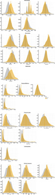
2.3 Preparatory internet experimentTo characterize stimuli with regard to their potential to elicit mind-wandering and influence the quality of thoughts, stimuli were evaluated in an internet experiment with n = 135 included participants, each completing two trials per emotion (joy, peaceful, nervous, sad). Thus, across all participants, 270 valid trials were gathered for each emotion. Participants listened to the music stimuli with the instruction to close their eyes and relax. After each stimulus, thought probes were collected, consisting of 10 questions. These questions were identical to a previous study (Koelsch et al., 2019) and are listed in Data S3. The questions assessed the control of the focus of attention, intensity of mind wandering, level of meta-awareness, affective valence of thoughts, arousal of thought content, self-referentiality, reference to other people, time relation, as well as relevance of thought contents to current concerns of the participant's life. Mind-wandering was assessed with the answer “yes/no” in response to the item “Were your thoughts completely focused on the music?”, and occurred with a similar frequency across all four music conditions (during joyful stimuli in 198 out of the 270 trials, during peaceful stimuli in 210, during nervous stimuli in 195, and during sad stimuli in 203 trials). Importantly, the valence of thoughts (as assessed by the item “Was what you were thinking about rather negative or positive?”) was influenced by the valence of the music, such that positive music evoked thoughts with more positive valence, and negative music evoked thoughts with more negative valence (F[1,103] = 76.91, p < .00001, η2 = .43, observed power: 1.0; see Figure 1a and Data S4 for details). Moreover, the arousal of thought contents (as assessed with the item “Was what you were thinking about making you rather calm or agitated?”) was higher during fast compared to slow music (F[1,103] = 249.88, p < .00001, η2 = 0.71, observed power: 1.0; see Figure 1a for details), and higher during negative compared to positive music (F[1,103] = 44.17, p < .00001, η2 = .30, observed power: 1.0). No other effects nor any interactions were observed for these variables, nor for any of the other collected items. Thus, our selected stimulus material had a strong effect on the valence and arousal of thoughts.

Valence and arousal of thought contents during mind-wandering. The yellow-framed boxes indicate results of the preparatory internet experiment (a), green-framed boxes indicate results of the fMRI experiment (b). Blue disks represent positive-sounding music (joy, peaceful), red disks negative-sounding music (nervous, sad), dark disk colors indicate fast music (joy, nervous), and light disk colors indicate slow music (peaceful, sad). Black disks indicate mean ratings of rest blocks in the fMRI experiment (no rest blocks were administered in the internet experiment). Data were z-transformed (separately for the preparatory internet experiment and the fMRI experiment). In both experiments, the valence of thoughts was higher for positive than negative-sounding music, and the arousal of thoughts was higher for fast than for slow music. Note: ***p < .001; **p < .01; *p < .05
2.4 fMRI session: ProcedureIn the fMRI experiment, music stimuli were concatenated (separately for each emotion condition) and presented in blocks, resulting in four music blocks (joy, peaceful, nervous, sad). In addition, the experimental paradigm included two rest blocks. Each block had a duration of 5 min. Ordering of the six blocks was pseudo-randomized (such that the second rest block would never follow directly the first rest block) and counterbalanced across participants. The task for the participants was to relax (in both the rest and the music blocks), and to listen to the music (in the music blocks). At the beginning of each block, participants were asked to keep their eyes closed until the end of the block, when a beep tone signaled to open the eyes and commence the rating procedure. Then, 10 questions were presented visually, and participants responded to each question on a six-point scale via two fMRI-compatible response buttons (one in each hand), using their index fingers. The direction of the scales was counterbalanced across trials, to exclude potential motor preparation during the music blocks and thus potential response bias. The wording of the questions was identical to a previous study (Koelsch et al., 2019) and the preparatory internet experiment (Data S3). The rating procedure was practiced before the fMRI session.
2.5 ApparatusMRI acquisition was carried out with a 3.0 T MRI machine (General Electric, Chicago, IL) at the radiology department of the Haukeland University Hospital in Bergen, Norway. A 32-channel phased-array head coil was used. A three-dimensional T1-weighted, high-resolution anatomical image was acquired for each participant using a magnetization-prepared rapid acquisition gradient echo (MP-RAGE) sequence (repetition time [TR] 2,250 ms, echo time [TE] 30 ms, voxel size 1 × 1 × 1 mm). A gradient echo, echo-planar pulse sequence (1172 functional volumes; TR 2250 ms; TE 30 ms; 3 mm slice thickness; 37 axial, sequential, top-down slices with a 0.6 mm gap; flip angle = 70°; matrix = 64 × 64; FOV = 192 × 192 mm) sensitive to BOLD contrast was used to acquire functional data. Additionally, the acquisition window was tilted by a 30° angle to the intercommissural plane (AC-PC); this procedure is helpful in reducing the susceptibility to artifacts in areas such as the orbitofrontal cortex and temporal lobe (Weiskopf, Hutton, Josephs, Turner, & Deichmann, 2007). Visual stimuli were presented via an in-room monitor, and audio-stimuli were presented via MRI compatible headphones (model NNL HP-1.3, NordicNeuroLab, Bergen, Norway) with a flat range response of 8–35,000 Hz and an external noise attenuation of an A-weighted equivalent continuous sound level of 30 dB.
2.6 Behavioral data analysisBehavioral data obtained in the preparatory internet survey and during the fMRI experiment were analyzed using SPSS 26 (IBM, Armonk, NY). Only data from 29 participants of the fMRI were analyzed because of data loss due to technical reasons.
2.7 Functional MRI data analysisDatasets were preprocessed using standard methods implemented in SPM12 (Wellcome Trust Centre for Neuroimaging, London, UK; RRID:SCR_007037) and the MIT connectivity toolbox (Connectivity Toolbox; RRID:SCR_009550), consisting of slice-time correction, realignment and reslicing of functional volumes, artifact detection (using the Artifact Detection Tools, RRID:SCR_005994), denoising via regression of average white matter timeseries, average CSF timeseries, 24 Volterra expansion movement parameters and scan-nulling regressors (Lemieux, Salek-Haddadi, Lund, Laufs, & Carmichael, 2007). Normalization to the sample's optimal template and from that to the ICBM MNI template (Fonov et al., 2011) was performed in a single step using SyGN (Tustison et al., 2013). Spatial smoothing using a 3D Gaussian kernel and a filter size of 6 mm at FWHM, as well as temporal high-pass filtering with a cut-off frequency of 1/90 Hz, were performed in a single step using the Leipzig Image Processing and Statistical Inference Algorithms (LIPSIA v2.2.7, RRID:SCR_009595). Voxel-wise eigenvector centrality mapping (ECM), an advanced graph theory method accounting for whole-brain functional connectomics (for illustration of eigenvector centrality see Data S1), was computed based on positive correlations, similarly as in previous studies (e.g., Koelsch & Skouras, 2014; Skouras et al., 2019; Taruffi et al., 2017), yielding ECM images for each condition and for each subject. (Note that both positive and negative conditions contained both arousing and relaxing stimuli, and that the overall level of arousal was balanced between positive and negative stimuli). ECM images were gaussianized voxel-wise across all subjects (van Albada & Robinson, 2007), to enable second-level parametric inference.
To compute the contrast between two music conditions (positive [joy and peaceful] vs negative [sad and nervous]), ECM images from all subjects were entered into a second-level general linear model and a paired-samples t-test was performed, resulting in a z-score map. Clusters with significant differences in eigenvector centrality between the two conditions were identified following correction for multiple comparisons by using a combination of single-voxel probability thresholding as well as cluster-size and cluster-z-value thresholding, through 10,000 iterations of Monte Carlo simulations. The initial cluster threshold of randomly generated maps of z-values was set to a probability level equivalent to a one-tail significance level of p = .01 (due to the replicatory nature of the study). The Monte Carlo simulations accounted for anatomical priors through hemispheric symmetry and generated thresholds for cluster sizes and peak z-values based on the initial threshold and the specific geometrical properties of the images (i.e., number of voxels, voxel size, spatial extent and spatial smoothness) to control for false positives and obtain the final activation maps corrected for multiple comparisons at the p = .05 level of significance (Lohmann et al., 2010; van Albada & Robinson, 2007).
2.8 Valence-specific functional connectivity analysisThe ECM results indicated a cluster in the posterior cingulate sulcus at the group level for the contrast negative versus positive music (replicating the finding of our previous study; Taruffi et al., 2017). This cluster was then used as a seed to compute its standardized functional connectivity, via Fisher's r to z transformation, with each gray matter voxel across the whole brain for each subject, for each condition (positive and negative) separately. On the second level, contrasts of positive and negative functional connectivity maps were computed via a paired-samples t-test, to obtain the valence-specific (e.g., stronger during negative than positive) functional connectivity of the seed cluster. Clusters with significant differences between positive and negative stimuli, in relation to the seed cluster, were identified following correction for multiple comparisons, performed identically as for the ECM analysis, with the exception of setting the corrected level of significance at p = .001 (to protect against false positives).
3 RESULTS 3.1 Behavioral dataDuring the rest blocks, participants rated their mind-wandering (conceptualized for this experiment as task-unrelated thinking) with the item “How much were you thinking about the experiment versus something else?” on a scale from 1 to 6) on average as moderate (M = 4.1, SD = 1.4). During the music blocks, participants also reported moderate mind-wandering (joy: M = 3.2, SD = 1.2; peaceful: M = 3.9, SD = 1.2; sad: M = 3.3, SD = 1.3; nervous: M = 3.2, SD = 1.0). Although mind-wandering was nominally strongest during peaceful music, this difference (compared to the other music conditions) was not significant (corrected for multiple comparisons). Compared with rest, mind-wandering was weaker during joy, sad, and nervous music (all p < .05, corrected for multiple comparisons), but not during peaceful music (p > .05). Importantly, replicating the results of our preparatory internet experiment (see Section 2), the valence of thought contents was significantly more positive during positive (joy, peaceful) than negative (nervous, sad) music (F[1,24] = 4.73, p = .04, η2 = .17, observed power: .55; see Figure 1b and Data S5). One-sided tests showed that, compared to rest, thought contents were significantly more positive during positive music (F[1,26] = 5.83, p < .05, η2 = .18, observed power: .64), and tended to be more negative during negative music (F[1,26] = 1.77, p < .1). The arousal of thought contents was higher during fast (joy, nervous) than slow (peaceful, sad) music (F[1,26] = 8.99, p = .006, η2 = .3, observed power: 0.82), but importantly (and contrary to the pilot experiment) there was no significant difference in the arousal of thought contents between positive and negative music (p = .07). Compared to rest, the arousal of thought contents was higher during fast music (F[1,26] = 3.95, p < 0.05 one-sided, η2 = .13, observed power: 0.48). No other main effects or interactions were observed for any of the other items. In summary, mind-wandering emerged during all experimental blocks, the valence of thoughts was more positive during positive music, and the arousal of thought contents was higher during fast music (but did not differ between positive and negative music).
3.2 Eigenvector centrality mappingGiven that mind-wandering emerged during all music conditions, we first investigated whether a similar eigenvector centrality pattern emerged during music and rest. We observed that the eigenvector centrality maps (ECMs) of the rest blocks showed a striking similarity with the ECMs of each of the music blocks (joy, peaceful, nervous, and sad): The ECM clusters strongly overlapped in all conditions (Figure 2a), with peak coordinates across all conditions located within the same or adjacent voxels. This remarkable overlap is demonstrated in the conjunction analysis of the ECMs across all conditions (Figure 2b): Any colored voxel in Figure 2b indicates that this voxel had a relatively high eigenvector centrality value in each of the six blocks (two rest blocks, and four music blocks). No other ECM-clusters were observed in the two rest blocks, and no significant differences emerged in a direct contrast between any of the music blocks on the one hand, and the two rest blocks on the other (i.e., none of the music conditions differed significantly from the rest condition). These results indicate that the resting-state network (as observed during rest) was also active during music (consistent with the observation that both rest and music conditions evoked mind-wandering, as indicated by the behavioral data).

Eigenvector Centrality Mapping. (a) The eigenvector centrality maps (ECMs) for the six experimental blocks (ordering of stimulus and rest blocks was counterbalanced across subjects; rating procedures at the end of each block were not included in the analysis). The locations of centrality maxima elicited across all six blocks were remarkably similar. This similarity is demonstrated in the conjunction analysis of the six eigenvector centrality maps (b). Regions with high eigenvector centrality overlap were found in the “midline core” (yellow) of the default mode network (DMN), the “dorsal medial prefrontal cortex subsystem” (blue), and the “medial temporal lobe subsystem” (green, note that the PHC clusters extend outside the DMN into fusiform areas). Additional regions with high eigenvector centrality (orange) include the extrastriate medial occipital cortex, midcingulate cortex, lateral parietal lobe, and temporal cortex. Images are shown in neurological convention. The blue cross-hairs indicate the coordinates of the slices shown. Only voxels with eigenvector centrality values ≥0.41 are shown, corresponding to the top tertile of centrality values (note that the centrality values do not indicate statistical significance). Coordinates refer to MNI space. ACC, anterior cingulate cortex; FUS, fusiform cortex; HF, hippocampal formation; OFC, orbitofrontal cortex; PCC, posterior cingulate cortex; PHC, parahippocampal cortex; TPJ, temporoparietal junction; vmPFC, ventro-medial prefrontal cortex
Notably, this resting-state network, as assessed using ECM, is reminiscent of the Default Mode Network (DMN), as typically assessed using independent component analysis (ICA): Regions with high eigenvector centrality overlap with the “midline core” of the DMN (yellow in Figure 2b), with the “dorsal medial prefrontal cortex subsystem” of the DMN (blue in Figure 2b), and the “medial temporal lobe subsystem” of the DMN (green in Figure 2b). Additional regions with high eigenvector centrality observed in the present study (orange in Figure 2b) include the midcingulate cortex (MCC), extrastriate medial occipital cortex, lateral parietal lobe, and temporal cortex. Interestingly, as can be seen in Figure 2a, the areas with the highest eigenvector centrality values were not part of the DMN (in particular visual cortex, and MCC).
3.3 ECM contrastsWe then investigated differences in ECMs between positive (joy & peaceful) and negative (nervous & sad) music (note that the average tempo was identical for positive and negative music, leading to comparable arousal for positive and negative stimuli). Regions in which eigenvector centrality differed between positive and negative music are shown in Figure 3 (for details see Table 1; these regions were also revealed in an analogous analysis including age, sex, and framewise displacement as covariates, see Data S6). Higher centrality values during negative (compared to positive) music were indicated in the upper bank of the posterior cingulate sulcus, extending medially into the paracentral lobule (see also left inset in Figure 3). According to the four-region model of the cingulate cortex proposed by Palomero-Gallagher et al. (2009), this region likely corresponds to area 23c of the posterior cingulate cortex (PCC), which is located within, and in the close vicinity, of the posterior cingulate sulcus (see middle inset in Figure 3). The PCC thus extends into, and beyond, the upper bank of the cingulate sulcus, bordering anterior-superiorly on area 5 (subfield 5 Ci). Likewise, a connectomic analysis of area 23c shows that white matter tracts of area 23c originate from within, and around, the posterior cingulate sulcus (see right inset in Figure 3). To the best of our knowledge, no anatomical probability map of area 23 is available. For example, this area has not been included yet in the SPM Anatomy toolbox (Eickhoff et al., 2005). Using the Anatomy toolbox (with its option “Overlap between structure and function”) we found that the probability for the cluster being located in area 5 is merely 19%, rendering it unlikely that neural activity in our cluster originated (only) from area 5.
 Contrast of eigenvector centrality maps. The top panel shows the ECM contrast of positive (joy & peaceful) versus negative (nervous & sad) music, corrected for multiple comparisons. The blue cluster indicates that, during negative-sounding music (associated with negative valence of thought contents), higher network centrality emerged in the posterior cingulate sulcus (area 23c of the posterior cingulate cortex). During positive music (associated with positive thought contents) higher centrality emerged in the dorsolateral premotor cortex (yellow-red clusters). Bottom panel: The left inset shows a coronal view of the cluster in area 23c, illustrating that the cluster includes the upper bank of the posterior cingulate sulcus. The middle inset shows the receptor-architectonic parcellation of the posterior cingulate cortex according to Palomero-Gallagher et al. (2009; the blue and violet colors indicate sub-regions of the PCC). Note that area 23c covers both the lower and the upper banks of the cingulate sulcus. The black arrow indicates the approximate location of the ECM cluster in area 23c. The right inset shows white matter tracts of area 23c in orange, according to the connectomic atlas by Baker et al. (2018; the white arrow indicates the approximate location of the ECM cluster in area 23c). Images are shown in neurological convention, coordinates refer to MNI space, the color-bars indicate z-values. CC, corpus callosum
TABLE 1.
Contrast of eigenvector centrality maps (ECMs)
ECM contrast of positive vs. negative music stimuli
Area
Vol. (mm3)
z-value (mean ± SD)
z-value (max)
MNI-coord.
Post. cingulate sulcus (area 23c)
432
−2.70 ± 0.38
−3.72
−3, −39, 58
SFGp (BA6 left)
999
2.70 ± 0.34
3.74
−18, 0, 76
SFGp (BA6 right)
2,133
2.81 ± 0.50
4.56
24, 3, 67
Note: Results of the ECM contrast of positive (joy & peaceful) versus negative (nervous & sad) music. Negative z-values indicate higher centrality during negative than positive stimuli (and vice versa). Results were corrected for multiple comparisons (p < .05), using 10,000 Monte Carlo permutations. BA: Brodmann area; SFGp: posterior superior frontal gyrus.
Contrast of eigenvector centrality maps. The top panel shows the ECM contrast of positive (joy & peaceful) versus negative (nervous & sad) music, corrected for multiple comparisons. The blue cluster indicates that, during negative-sounding music (associated with negative valence of thought contents), higher network centrality emerged in the posterior cingulate sulcus (area 23c of the posterior cingulate cortex). During positive music (associated with positive thought contents) higher centrality emerged in the dorsolateral premotor cortex (yellow-red clusters). Bottom panel: The left inset shows a coronal view of the cluster in area 23c, illustrating that the cluster includes the upper bank of the posterior cingulate sulcus. The middle inset shows the receptor-architectonic parcellation of the posterior cingulate cortex according to Palomero-Gallagher et al. (2009; the blue and violet colors indicate sub-regions of the PCC). Note that area 23c covers both the lower and the upper banks of the cingulate sulcus. The black arrow indicates the approximate location of the ECM cluster in area 23c. The right inset shows white matter tracts of area 23c in orange, according to the connectomic atlas by Baker et al. (2018; the white arrow indicates the approximate location of the ECM cluster in area 23c). Images are shown in neurological convention, coordinates refer to MNI space, the color-bars indicate z-values. CC, corpus callosum
TABLE 1.
Contrast of eigenvector centrality maps (ECMs)
ECM contrast of positive vs. negative music stimuli
Area
Vol. (mm3)
z-value (mean ± SD)
z-value (max)
MNI-coord.
Post. cingulate sulcus (area 23c)
432
−2.70 ± 0.38
−3.72
−3, −39, 58
SFGp (BA6 left)
999
2.70 ± 0.34
3.74
−18, 0, 76
SFGp (BA6 right)
2,133
2.81 ± 0.50
4.56
24, 3, 67
Note: Results of the ECM contrast of positive (joy & peaceful) versus negative (nervous & sad) music. Negative z-values indicate higher centrality during negative than positive stimuli (and vice versa). Results were corrected for multiple comparisons (p < .05), using 10,000 Monte Carlo permutations. BA: Brodmann area; SFGp: posterior superior frontal gyrus.
Compared with rest, centrality values of the cluster in the posterior cingulate sulcus were higher during negative music (max z = 2.87), and did not differ between rest and positive music. Thus, negative music increased the functional centrality of neurons in the posterior cingulate sulcus compared to both rest and positive music. Higher eigenvector centrality values during positive (compared to negative) music were indicated in the dorso-lateral premotor cortex bilaterally (area 6). Contrary to our previous study (Taruffi et al., 2017), no significant differences between positive versus negative music were observed in the vmPFC.
3.4 Data-driven hypothesis generation and functional connectivity analysisThe ECM contrast analysis revealed that the centrality of the posterior cingulate sulcus (area 23c of the PCC), varies depending on the valence of music-evoked thoughts. To aid the interpretation of this finding, we (first) explored the functional significance of area 23c using meta-analytic data, then (second) investigated the functional connectivity of this region, also using meta-analytic data, and finally (third) computed the functional connectivity of area 23c using the fMRI data of the present study, comparing the functional connectivity of area 23c between positive and negative music in order to specify whether the functional connectivity of area 23c is modulated by emotions. These three steps are described in more detail in the following.
First, we identified the meta-analytic activation pattern associated with the peak coordinate of the ECM cluster observed in area 23c (listed in Table 1) using the Neurosynth platform (neurosynth.org; Yarkoni, Poldrack, Nichols, Van Essen, & Wager, 2011). The top associated label (out of 525 labels), was “painful” (posterior z = 5.64), followed by the label “pain” (posterior z = 5.14). This indicates a role of area 23c in pain.
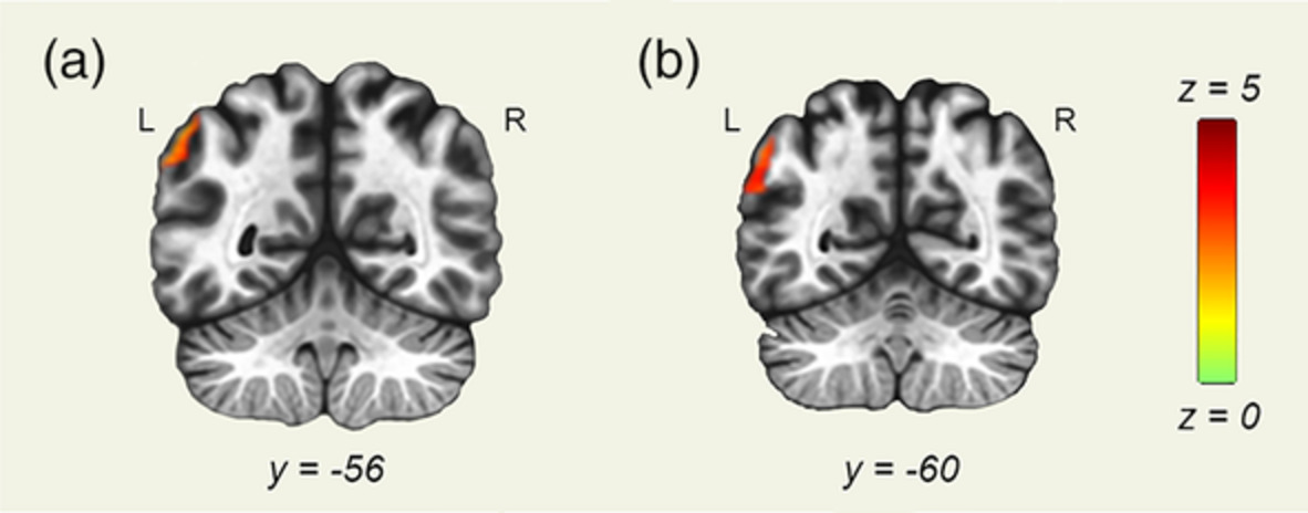
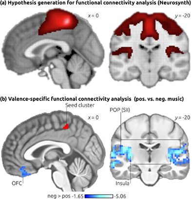
Second, we accessed the functional connectivity map generated by Neurosynth using our peak coordinate in area 23c as a seed coordinate (Neurosynth provides voxel-based resting-state functional connectivity analyses based on a pool of 1000 fMRI datasets). That map is shown in Figure 4a, indicating functional connectivity of area 23c during rest with lateral and medial (primary) somatosensory cortex (SI), MCC, secondary somatosensory cortex (SII) in the parietal operculum (POP), and posterior (granular) insular cortex. (Notably, as we will discuss in more detail further below, two of these regions, namely SII and insula are among the four “core regions consistently activated by pain”; Xu et al., 2020).

Functional connectivity analysis. To generate hypotheses for a functional connectivity analysis of area 23c, we accessed the resting-state functional connectivity map of the peak coordinate of the ECM cluster in the posterior cingulate sulcus (area 23c) as provided by the Neurosynth platform (see main text for details). This analysis indicated functional connectivity of area 23c with MCC, lateral and medial SI, SII, and insular cortex (a). Then, a valence-specific functional connectivity analysis was computed with the data obtained in our fMRI experiment (b), using the ECM cluster in area 23c as the seed region (illustrated by the red cluster). Results showed stronger functional connectivity of area 23c during negative compared with positive music (indicated in blue) with secondary somatosensory cortex (SII), insula, and OFC. Results are corrected for multiple comparisons (p < .001), using 10,000 Monte Carlo permutations. Images are shown in neurological convention, coordinates refer to MNI space, the color-bar in (b) indicates z-values. OFC, orbitofrontal cortex; POP, parietal operculum
Third, based on these observations, we compared the functional connectivity of area 23c with these regions (SI, SII/POP, MCC, posterior insula) between the two conditions (positive vs negative) of the present experiment, hypothesizing that area 23c would show stronger functional connectivity with these regions during negative, compared with positive, music. Results of this valence-specific functional connectivity analysis are shown in Figure 4b. In line with our hypothesis, area 23c showed significantly stronger functional connectivity during negative compared with positive music with secondary somatosensory cortex (SII/POP) and insula. Additional regions with stronger functional connectivity during negative compared to positive music were observed in the medial orbitofrontal cortex (mOFC), auditory cortex, and the anterior hippocampal formation (for details see Table 2). No significant valence-specific functional connectivity was observed with SI or MCC.
TABLE 2. Valence-specific functional connectivity analysis Area Vol. (mm3) z-value (mean ± SD) z-value (max) MNI-coord. (a) Contrast of functional connectivity maps: Negative > positive music stimuli L auditory cortex (core and belt regions) 29,916 −2.96 ± 0.48 −5.06 −60, −12, 7 POP −4.44 −45, −15, 21 STGp −4.21 −66, −21, 12 Post. insula −4.24 −36, −18, 6 Mid insula −4.10 −36, 0, −6 Ant. Insula −3.81 −27, 15, −15 Post. STS −3.29 −45, −48, 15 Ant. Hippocampus −3.04 −27, −12, −21 R post. Insula 22,113 −2.89 ± 0.42 −4.43 42, −12, 4 Mid insula −3.99 45, 0, 3 POP −3.97 54, −21, 15 Post. STS −3.70 51, −3, 6 R parahipp. cortex/collateral sulcus 4,158 −2.71 ± 0.33 −3.63 27, −45, −2 L parahipp. cortex/collateral sulcus 4,374 −2.85 ± 0.41 −3.95 −24, −45, −8 L OFC (vmPFC) 3,861 −2.60 ± 0.24 −3.53 −9, 27, −23 (b) Contrast of functional connectivity maps: Positive > negative music stimuli R cerebellum 6,210 2.70 ± 0.34 3.91 12, −90, −20 Note: The table lists the results of the functional connectivity analysis of the ECM cluster in the posterior cingulate sulcus (area 23c) as seed region (illustrated by the red cluster in Figure 4b): the results of the contrast negative > positive are listed in (a), and results of the opposite contrast are listed in (b). Results indicate stronger functional connectivity of area 23c during negative (compared with positive) music with auditory cortex, SII, insula, the hippocampal formation, and OFC. Results were corrected for multiple comparisons (p < .001), using 10,000 Monte Carlo permutations. Abbreviations: ant., anterior; L, left; OFC, orbitofrontal cortex; parahipp, parahippocampal; POP, parietal operculum; post, posterior; R, right; STS, superior temporal sulcus; vmPFC, ventro-medial prefrontal cortex. 3.4.1 Replication of valence-specific functional connectivityFinally, we aimed at replicating the results of the valence-specific functional connectivity analysis (as shown in Figure 4b and listed in Table 2) using the data from our previous study (Taruffi et al., 2017) with music evoking sadness or joy, also using area 23c as seed region. Using the same preprocessing and functional connectivity analysis pipeline described above for the main experiment (including the same seed region), the contrast maps of the valence-specific functional connectivity (joy vs. sad) indicated local maxima in both left (z = −3.30, MNI coordinate: −42, −18, 21) and right (z = −2.76, MNI coordinate: 36, −21, 21) parietal operculum (with the cluster in the right POP extending into the posterior insula), as well as in the mOFC (z = −2.55, MNI coordinate: −6, 39, −18). In all of these stru
留言 (0)