
記住我

Gliomas are the most common primary intracranial tumor, representing 81% of malignant primary brain tumors (Ostrom et al., 2013, 2014). Brain tumors within language eloquent regions can cause aphasia depending on tumor size, edema, and localization per se. However, the localization of language eloquent fiber tracts shows significant interindividual variability, especially in patients suffering from lesions in eloquent brain areas. Understanding the mechanisms of aphasia in glioma patients will improve the understanding of the neural function and structural plasticity, which is essential for preserving brain functions in individualized tumor treatment concepts.
Preoperative identification of language-related regions is essential to preserve functionality during tumor resection in eloquent locations. Navigated transcranial magnetic stimulation (nTMS) and functional magnetic resonance imaging (fMRI) have both been widely applied preoperatively to identify the individual language-related regions. However, fMRI lacks precision, especially in the vicinity of brain lesions based on inaccuracies due to pathological tumor vascularization (Lin et al., 2017; Silva, See, Essayed, Golby, & Tie, 2018). nTMS has shown to be highly predictive regarding negative stimulation sites, and comparisons to the gold standard of intraoperative direct cortical stimulation (DCS) showed a high accuracy of nTMS (Ille et al., 2015a, 2015b; Picht et al., 2013). Therefore, nTMS mapping of motor- and language-eloquent brain areas is routinely used preoperatively to identify language-related fiber tracts and for preoperative risk assessment combined with fiber tracking (FT).
FT is based on the fusion of data on functional brain areas such as cortical nTMS mapping data and subcortical structural tractography shown by diffusion tensor imaging (DTI; Ille et al., 2015a, 2015b). Previous studies have shown that language function is separated into cortical and subcortical collaborating networks (Hagoort, 2019; Henderson, Choi, Lowder, & Ferreira, 2016; Lohmann et al., 2010; Xiang, Fonteijn, Norris, & Hagoort, 2010). For instance, the temporo-frontal networks are assigned to tasks on semantic and syntactic processing (Friederici, Ruschemeyer, Hahne, & Fiebach, 2003).
Connectomes are used to represent the functional composition of nodes—relevant brain areas as mapped by nTMS—and their connections as visualized by DTI within the network. The combination of graph theory, nTMS, and connectome analysis of DTI data is a novel multidisciplinary paradigm considering the brain as a complex network of individual components interacting through continuous communication. Thereby it offers further insight into both local and global effects of gliomas on these complex networks (Hart, Romero-Garcia, Price, & Suckling, 2019). Previous studies using nTMS-based FT only focused on single neural tracts in patients with glioma-induced aphasia (GIA; Sollmann et al., 2020). However, recent studies have shown that gliomas have a global impact on the whole brain (Derks et al., 2017; Hart et al., 2019). Therefore, there is a necessity of analyzing global nTMS mapping-based networks to investigate neuroplasticity and remodulation mechanisms related to aphasia.
As shown by graph theory in previous studies, the organization of cerebral structures is compatible with the hypothesis that the brain evolved to maintain the dynamic balance between maximization of the efficiency in transferring information and minimization of connection cost (Betzel et al., 2014; Bullmore & Sporns, 2009; Gargouri et al., 2016). Graph-based network analysis enables to derive properties of the brain's “connectome” and delivers information on the topological architecture of human brain networks, such as average degree (AD), global efficiency (EG), and local efficiency (EL), which has already been introduced for functional MRI (Betzel et al., 2014) and EEG analysis (Gu et al., 2020). AD is the basic character to present the intensity of connections across all nodes in the network (Cohen & D'Esposito, 2016). EG measures the capacity in parallelly transferring and comprehensively processing information (Wang, Zuo, & He, 2010). EL indicates the fault-tolerant capacity of the network and the efficiency of the communication between immediate neighbors of the local node (Wang et al., 2010). Previous studies on tractography networks in glioblastoma patients demonstrated significant differences in tract volumes based on nTMS positive and negative mapping sites (Sollmann et al., 2020). However, graph theory metrics and their differences have not yet been measured to analyze the impact of tumors on cerebral structural network properties. Further investigations are still lacking to distinguish the network based on eloquent language regions identified by nTMS from the left and right hemispherical networks.
This study aimed to evaluate the global and local properties of function-specific connectomes derived from nTMS language mapping. Graph properties of aphasic and nonaphasic glioma patients of the resulting connectomes based on positive and negative nTMS mapping regions were analyzed and correlated with different states of aphasia. Connectomes were constructed and analyzed based on tractography thresholding at different levels to assess the robustness and efficacy of networks.
2 MATERIALS AND METHODS 2.1 EthicsThe current study was performed in accordance with the Declaration of Helsinki and its later amendments, and its protocol was approved and supervised by the local ethics board (registration number: 222/14, 338/16, 2793/10, 5811/13, 223/14, and 336/17). Written informed consent was obtained from all patients before enrolling in the current study.
2.2 Study eligibilityThe following inclusion criteria were considered: (a) age above 18 years, (b) mother tongue German, (c) primary diagnosis being glioma with following pathological confirmation, (d) tumor within a left perisylvian region adjacent to the arcuate fasciculus-related cortical and subcortical regions, (e) no previous cranial surgery, and (f) written informed consent. Patients with contraindications for MRI or nTMS examinations such as pregnancy, intracranial metallic implants, cochlear implants, and pacemakers were excluded. Overall, 30 patients with no aphasia (NA) and 30 patients with GIA were considered eligible from our database of patients undergoing nTMS language mapping in our department from 2016 to 2019.
2.3 Data collection and proceduresFor all patients, preoperative MRI (Achieva 3T, Philips Medical System, Netherlands BV) images were acquired, including DTI scans (TR/TE: 5,000/78 ms, voxel size of 2 × 2 × 2 mm3, 32 diffusion gradient directions, b value 1,000 s/mm2) and a 3D T1-weighted gradient-echo sequence with and without intravenous contrast agent (TR/TE: 9/4 ms, 1 mm3 iso-voxel, Dotagraf 0.5 mmol/ml, produced by Jenapharm GmbH & Co. KG, Jena, Germany, phase-encoding at rostral–caudal direction) in our neuroradiological department for quality control and stable scanning.
2.4 Language mapping and aphasia testingThe aphasia level testing was performed according to the Aachener aphasia test (AAT) for both groups (Biniek, Huber, Glindemann, Willmes, & Klumm, 1992). The handedness test was conducted according to Edinburgh Handedness Inventory (EHI; Oldfield, 1971).
nTMS language mapping was performed following the standard protocol used in clinical routine using a Nexstim eXimia NBS system (version 5.1.1; Nexstim Plc, Helsinki, Finland; Krieg et al., 2017; Sollmann, Fuss-Ruppenthal, Zimmer, Meyer, & Krieg, 2018). Contrast-enhanced T1 weighted images were used for neuronavigation. Stimulator output was set at 100% of the individual resting motor threshold. Stimulation was performed using 5 pulses at 5 Hz on individually predefined 46 targets according to the cortical parcellation system (Krieg et al., 2017; Sollmann et al., 2018). nTMS language mapping consisted of a baseline session without stimulation and a stimulating session with stimulation during the patient performing an object naming task (ONT), during which audios and videos were recorded for post-hoc analysis. Each naming performance with stimulation was compared with the individual baseline to identify naming errors, which were categorized into five types: no-response, performance, phonological paraphasias, semantic paraphasias, and neologism (Krieg et al., 2017; Sollmann et al., 2018). Stimulated sites with naming errors (positive nTMS stimulation regions [POS]) and without naming errors (negative nTMS stimulation regions [NEG]) were separated and exported as DICOM (digital imaging and communications in medicine) format files for further analysis. Mapping results were analyzed by both technicians and neurosurgeons. Durations of language mapping examinations were about 30 min per case.
2.5 Network constructionContrast-enhanced T1 images were skull-striped using HD-Bet (Isensee et al., 2019). In the next step, they were linearly co-registered to b0 images derived from the DTI data set, and the POS and NEG stimulation sites derived from nTMS language mapping were transferred into the DTI space. The anatomic atlas template AAL90 (Tzourio-Mazoyer et al., 2002) was co-registered to the T1 image using the SyN algorithm from ANTs (https://github.com/ANTsX/ANTs; Avants, Epstein, Grossman, & Gee, 2008) and diffusion-weighted b1000 images were linearly registered to the b0 image. The gradient vector table was rotated accordingly and corrected for eddy currents (Figure 1). Finally, nTMS POS and NEG sites, as well as AAL90 atlas locations, were co-registered to the DTI space, and the total number of regions in the AAL90 anatomic template corresponding to POS or NEG points was counted for each subject.

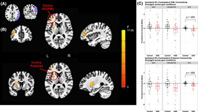
Workflow of the current study. This figure illustrates the process of network construction. DTI scans with 32 directions (A), T1 images with contrast (B), T1 images with contrast without skull and skin (C), the anatomic atlas template AAL90 (D), and nTMS language mapping images (E) were registered to a B0 image (F). A deterministic algorithm was used for fiber tracking after applying constrained spherical deconvolution (CSD). The minimal FA for each fiber to be visualized was identified, from which its visualization ratio (VR) was calculated. The fibers with VR values above the thresholds of 25% (G) and 50% VR (H) were respectively used to construct five matrices: Mwhole, matrix (M) derived from nodes from both hemispheres and edges (fibers) connecting them. Mleft and Mright, respective matrices with nodes from the left (Mleft) or the right hemisphere (Mright) and intra-hemispheric edges (fibers). Mpos and Mneg, matrix with nodes from the positive language mapping regions and edges from their corresponding edges (fibers), and matrix with nodes from the negative language mapping regions and edges from their corresponding edges (fibers)
Next, whole-brain tractography was conducted through the Python library DIPY (Version 1.2.0, https://dipy.org; Garyfallidis et al., 2014), during which each voxel in the brain was used as region of interest (ROI; Figure 1). Then, constrained spherical deconvolution (CSD) was performed on the dataset (Tournier, Calamante, & Connelly, 2007). In the next step, a deterministic algorithm was applied to tractography with fractional anisotropy thresholds (FAT) starting from 0.0 continuously increased by 0.01 with a fiber length threshold (FLT) at 30 mm and stopping at a maximal FAT (FATmax). During this process, the maximal FA (famax) for every single fiber was identified. The following formula calculated the visualized ratio (VR) for each fiber: The tractography based on the fibers with VR above 25 and 50% were selected (Figure 1), from which the following five matrices (M) were constructed (Figures 2 and 3):
Mwhole: a matrix (M) at a size of 90 nodes × 90 nodes was created from both hemispheres based on the atlas AAL90 and their corresponding connections.
Mleft: a matrix based on nodes from the left hemisphere based on the atlas AAL90 and their corresponding connections at the size of 45 × 45.
Mright: a matrix based on nodes from the right hemisphere based on the atlas AAL90 and their corresponding connections at the size of 45 × 45.
Mpos: a matrix based on nodes from individual positive language mapping regions based on the atlas AAL90 and their corresponding connections.
Mneg: a matrix based on nodes from individual negative language mapping regions based on the atlas AAL90 and their corresponding connections.
Since brain size is variable among individuals, connections between two regions in matrices containing more than three fibers were considered as connected and binarized to 1, otherwise as they were considered as disconnected and binarized to 0 (Figure S1).
The tractography based on the fibers with VR above 25 and 50% were selected (Figure 1), from which the following five matrices (M) were constructed (Figures 2 and 3):
Mwhole: a matrix (M) at a size of 90 nodes × 90 nodes was created from both hemispheres based on the atlas AAL90 and their corresponding connections.
Mleft: a matrix based on nodes from the left hemisphere based on the atlas AAL90 and their corresponding connections at the size of 45 × 45.
Mright: a matrix based on nodes from the right hemisphere based on the atlas AAL90 and their corresponding connections at the size of 45 × 45.
Mpos: a matrix based on nodes from individual positive language mapping regions based on the atlas AAL90 and their corresponding connections.
Mneg: a matrix based on nodes from individual negative language mapping regions based on the atlas AAL90 and their corresponding connections.
Since brain size is variable among individuals, connections between two regions in matrices containing more than three fibers were considered as connected and binarized to 1, otherwise as they were considered as disconnected and binarized to 0 (Figure S1).

Comparison of mapping region counts. This figure presents counts of nTMS positive (Npos) and nTMS negative (Nneg) mapping regions for patients with no aphasia (NA) and glioma-induced aphasia (GIA). No significant intergroup differences were detected, while the intragroup analysis showed a lower count of Npos compared to Nneg in both groups (p < .001)

Nodes and connections from the whole brain, left hemisphere, and right hemisphere. This figure illustrates edges and nodes for matrices of the left hemisphere (Mleft—green), right hemisphere (Mright—yellow), and both hemispheres (Mwhole—purple) under different visualization ratios (VRs). The connections tracked in <10 patients (33.3%) are not shown to improve the visualization. A larger thickness of the edges indicates higher intragroup prevalence of the respective edges. Connection density in the no aphasia (NA) group was observed to be higher than that in the glioma-induced aphasia (GIA) group under both VRs
The connectome properties, including AD, EG, and EL, were assessed in each of the five binarized matrices under VR thresholds of 25 and 50%, respectively, using algorithms from the NetworkX 2.5 library (https://networkx.org/) in Python 3.7 (https://www.python.org/; Latora & Marchiori, 2001). The differences of each property calculated for 25% VR and 50% VR thresholds were recorded for each group as AD-diff, EG-diff, and EL-diff.
2.6 Connectome analysis and statistical analysisThe statistical analysis was performed using SPSS Statistic (IBM SPSS Statistics for Mac, Version 23.0. IBM Corporation, Armonk, NY) and GraphPad Prism (Version 8.4.3, San Diego, CA).
The chi-square test was applied to compare the demographic data between both groups, including handedness, pathological diagnosis, tumor locations, and gender. Furthermore, independent t-testing was applied to compare age and glioma size between the two groups.
For the analysis of mapping regions, the number of patients in each group with the same positively or negatively mapped regions was summarized, respectively. The intra-group proportion of being positively or negatively mapped was calculated for each region in the mapping template. The nonparametric test was used to analyze the difference of the mapping points between the NA and GIA groups.
ANCOVA testing with covariates was used to compare network properties between the NA and GIA groups, consisting of AD, EG, EL, AD-diff, EG-diff, and EL-diff. Correlation analysis was performed for different aphasia levels, properties, and the properties' alterations (AD-diff, EG-diff, and EL-diff).
Figures were created in MATLAB (Version R2016b, Company; authorized license to TUM) using BrainNet Viewer (Version 1.7; https://www.nitrc.org/projects/bnv/; Xia, Wang, & He, 2013). A level of significance at p < .05 was set for all tests. FDR correction was applied for multiple comparisons.
3 RESULTS 3.1 Demographic analysisSixty subjects were enrolled from the database of patients receiving treatments in our department between 2016 and 2019, consisting of 30 patients in the NA group and 30 patients in the GIA group. Age was 57.7 ± 15.1 years for the NA group and 63.9 ± 12.4 years for the GIA group (p = .093). There were no significant differences between the two groups regarding handedness, gender, and World Health Organization (WHO) grading (Table 1). FATmax was calculated for the NA (0.531 ± 0.065) and GIA (0.541 ± 0.063) groups. No significant differences were found between the two groups (p = .774).
TABLE 1. Comparisons on demographic data between NA and GIA group Items NA group GIA Group p Gender Male 6 11 .152 Female 24 19 Handiness Left 4 5 .718 Right 26 25 Pathology diagnoses I–III 11 6 .152 IV 19 2 Tumor sizes Average 2.4 4.7 .015a SD 2.6 4.3 Note: This table shows comparisons on patient characteristics between patients with NA (no aphasia) and GIA (glioma-induced aphasia). Average values and standard deviations (SD) of tumor sizes are shown additionally.Notably, glioma size in the NA group (2.4 ± 2.6 cm3) was significantly smaller than in the GIA group (4.7 ± 4.3 cm3; Table 1; p = .015). However, glioma size did not correlate with aphasia levels in the GIA group (p = .060, R = .249). As the tumor size was different between the two groups, glioma size was regarded as a covariate for the analysis of covariance (ANCOVA) in the following comparisons between the two groups for investigating the performance of structural networks. In the GIA group, the tumor affected the precentral gyrus, frontal inferior gyrus, and Rolandic operculum more often (Table S1).
3.2 Analysis of nTMS mapping regions TABLE 2. Intragroup proportion of each positive and negative language mapping region NA group GIA Group Proportion of each positive region Proportion of each negative region Proportion of each positive region Proportion of each negative region


Middle frontal gyrus: 93.3% (28 cases)
Precentral gyrus: 76.7% (23 cases)
Middle temporal gyrus: 76.7% (23 cases)
Postcentral gyrus: 70.0% (21 cases)
Superior frontal gyrus: 66.7% (20 cases)
Paracentral lobule: 100% (30 cases)
Fusiform gyrus: 100% (30 cases)
Precuneus gyrus: 100% (30 cases)
Lingual gyrus: 100 (30 cases)
Cuneus gyrus: 100% (30 cases)
Inferior frontal gyrus (orbital): 100% (30 cases)
Insula: 100% (30 cases)
Medial superior frontal gyrus: 96.7% (29 cases)
Superior occipital gyrus: 96.7% (29 cases)
Supplementary motor area: 86.7% (26 cases)
Heschl's gyrus: 86.7% (26 cases)
Rolandic operculum: 70.0% (21 cases)
Middle frontal gyrus: 90.0% (27 cases)
Precentral gyrus: 83.3% (25 cases)
Superior temporal gyrus: 80.0% (24 cases)
Middle temporal gyrus:76.7% (23 cases)
Postcentral: 70.0% (21 cases)
Angular gyrus: 70.0% (21 cases)
Supramarginal gyrus: 70.0% (21 cases)
Inferior frontal gyrus (opercular): 70.0% (21 cases)
Insula: 100% (30 cases)
Superior occipital: 100% (30 cases)
Inferior frontal gyrus (orbital): 100% (30 cases)
Precuneus gyrus: 100% (30 cases)
Fusiform: 100% (30 cases)
Cuneus gyrus: 100% (30 cases)
Lingual gyrus: 100% (30 cases)
Medial superior frontal gyrus: 96.7% (29 cases)
Paracentral lobule: 90.0% (27 cases)
Heschl's gyrus: 86.7% (26 cases)
Rolandic operculum: 66.7% (20 cases)
Note: This table shows results of the intragroup analysis on overlapping positive and negative regions identified in more than 20 patients (66.7%) with NA (no aphasia) and GIA (glioma induced aphasia) after registration to the AAL90 template. All mapping regions located were in the left hemisphere. The chi-square test was applied to identify mapped regions with significant differences between NA and GIA groups. The left supplementary motor area (SMA) was positively mapped in 4 cases of the NA group and 12 cases of the GIA group and with a significant difference between the NA and GIA group (K = 5.454, p = .019). The left angular gyrus is positively mapped in 13 cases of the NA group and 21 cases of the GIA group. The chi-square test shows NA patients were significantly more often positively to be mapped in the left angular gyrus (K = 4.343, p = .037).There were significantly less positive than negative stimulation sites in both the NA (Average counts of mapping regions: 16.600 (NEG) vs. 8.400 (POS); p < .001) and GIA (Average counts of mapping regions: 15.433 (NEG) vs. 9.567 (POS); p < .001) group (Table 2, Figure 2). More POS regions were found in the GIA group compared to the NA group (9.567 vs. 8.400, p = .083; Figure 2). In the GIA group, the total count of the POS regions (R = .226, p = .230) and NEG regions (R = −.226, p = .230) did not correlate with aphasia levels.
The middle frontal gyrus was most often mapped in both NA (28 patients; 93.3%) and GIA groups (27 patients; 90.0%) and without difference between the two groups (corrected chi-square test, p > .05; Table 2). Besides, the precentral gyrus, middle temporal gyrus, and postcentral gyrus were positively mapped in more than 20 cases in both NA and GIA groups (Table 2). Positive stimuli in the superior frontal gyrus were detected in 20 NA patients (66.7%) and 16 GIA patients (53.3%). Only in the GIA group, angular gyrus, supramarginal gyrus, and inferior frontal gyrus (Operculum) were positively mapped in more than 20 patients. Regarding the comparison of positive mapping regions in the left hemisphere between the two groups, most of them were without statistical difference between the two groups. However, the supplementary motor area (SMA; NA: 4 patients; GIA:12 patients; K = 5.454, p = .019) and angular gyrus (NA:13 patients; GIA:21 patients; K = 4.343, p = .037) showed the most remarkable difference between GIA and NA patients through chi-square testing (Table 2).
3.3 Intergroup network analysis 3.3.1 Analysis of ADUsing thresholding at 25% VR and 50% VR, AD from different matrices (Mwhole, Mleft, Mright, and Mneg) in the NA group was higher than AD in the GIA group. Mpos was slightly higher in GIA patients at 25% VR (2.073 vs. 2.076; Figures 3 and 4, Table 3), while Mleft was significantly higher in the NA group for 25% VR (5.430 vs. 4.827; p = .015) and 50% VR (1.833 vs. 1.434; p = .037). Mneg also showed a significant difference between groups under 25% VR (2.392 vs. 1.942; p = .042). The AD-diff in the NA group was higher, except for the AD-diff of Mpos (1.140 vs. 1.324; Figures 3 and 4, Table 3).

Nodes and connections based on nTMS mapping results. This figure illustrates nodes and edges for the matrices of nTMS positive mapping regions (Mpos, red) as well as nTMS negative mapping regions (Mneg, blue) in the left hemisphere under different VR setups. Fibers tracked in <3 patients (10%) are not shown as edges in the figures. A larger size of the nodes and edges indicates higher intragroup prevalence of the respective edges. There is a higher density of connections in patients without aphasia (NA) compared to patients with glioma-induced aphasia (GIA) for 50% VRs. Mpos shows a higher density of edges at 25% VR in the GIA group [A (25% VR) vs. B (25% VR)]
TABLE 3. Analysis on average degree, global, and local efficiency Items Mwhole Mleft Mright Mpos Mneg 25% VR AD NA group 7.635 5.430 5.833 2.073 2.392 GIA group 7.215 4.827 5.509 2.076 1.942 T-value 1.718 2.498 1.584 0.372 2.083 p-value .091 .015* .119 .712 .042* EG NA group 0.537 0.566 0.593 0.704 0.595 GIA group 0.520 0.533 0.578 0.705 0.532 T-value 2.406 2.513 1.422 0.327 2.034 p-value .019* .015* .161 .745 .047* EL NA group 0.717 0.716 0.732 0.682 0.633 GIA group 0.706 0.692 0.717 0.707 0.571 T-value 1.517 2.093 1.456 0.315 1.027 p-value .135 .041* .151 .754 .30950% VR
AD NA group 2.863 1.883 2.344 0.933 0.766 GIA group 2.457 1.434 2.126 0.753 0.523 T-value 1.776 2.139 1.176 1.592 1.669 p-value .081 .037* .117 .178 .101 EG NA group 0.330 0.297 0.371 0.437 0.227 GIA group 0.286 0.229 0.328 0.284 0.145 T-value 1.701 1.392 2.344 2.187 1.506 p-value .094 .169 .023* .033* .138 EL
留言 (0)