1 INTRODUCTION

According to the United Nations Office on Drugs and Crime, around 192 million of the global population regularly and recreationally (not for medical purposes) use cannabis.1 Regular and heavy cannabis use (HCU) is a modifiable risk factor for the development of mental illness2 and a widespread public health issue of mainly young adults.3-6 According to recent scientific evidence, there is a causal link between cannabis use and long-lasting common mental disorders (e.g., psychotic disorders6, 7 and substance-use disorders).4-6 In 2010, there were 2 million disability-adjusted life years (DALYs) attributable to cannabis dependence.3, 8 According to recent scientific evidence, there is a causal link between cannabis use and long-lasting common mental disorders (e.g., schizophrenia and other psychotic disorders).6, 7 One of the main hypotheses for psychotic disorders implicates different types of cannabis and a dysregulation (aberrant endogenous signalling) between the two main psychoactive components Δ-9-tetrahydrocannabinol (THC) and cannabidiol (CBD).6, 7 Furthermore, THC and CBD might differently interfere with the endocannabinoid and other neurotransmitter systems,9, 10 and hence, both substances have different acute-, residual- and long-term effects on affective, cognitive and sensorimotor functioning.11 On one side, THC can acutely increase positive mood12 and reduce anxiety at low doses.13 Further, higher doses of THC might increase the vulnerability of the 5-HT system and lead to depressive, anxiety and psychotomimetic effects (e.g., paranoia, dissociation and depersonalization) as well as impaired memory and attention.10, 14, 15 Additionally, long-term effects of cannabis on executive functions are seen in disturbed decision-making, concept formation and planning.11 On the other side, CBD might decrease the negative effects and perhaps increase the positive effects of THC,16 leading to antidepressant- and anxiolytic-like effects.17 The co-localization in the brain and interaction between endocannabinoid and opioid systems play a key role in pain processing, memory, reward and addiction.18-20 In particular, THC might suppress some opioid signs and symptoms.20 In turn, CBD may have an “anti-addictive” effect through its action on endocannabinoid, dopaminergic, serotonergic and opioidergic, systems.21, 22

Although both abnormal brain structure and function has been attributed to HCU, previous neuroimaging studies on HCU showed heterogeneous results mostly prevented through methodological constraints such as unimodal examination of patients with severe comorbid mental disorders. Therefore, it is unclear whether HCU is related to co-altered patterns of brain structure and function, or whether grey matter volume (GMV) and intrinsic neural activity (INA) convey unique and different aspects associated with HCU. Also, it is still unclear how HCU-related structural and functional brain abnormalities are coupled to different neurotransmitter systems. Given the importance of these questions, improving the understanding of the neurobiology underlying HCU is crucial to informing the development of new classes of treatment of both young individuals at high risk for developing a substance-use disorder (SUD).

In order to expand the extant knowledge on network abnormalities spanning across multiple imaging modalities in terms of joint function–structure alterations, which are related to HCU, this study had two major objectives: First, we predicted that there will be a difference in each modality-specific (i.e., brain structure or function) and intermodal (i.e., structure and function) systems comprising cognitive, reward-associated and sensorimotor networks between HCU and a control group without cannabis use. In particular, we chose amplitude of low-frequency fluctuations (ALFF) as primary measures of local intrinsic activity to facilitate comparability with previous research, particularly since several fMRI studies so far have shown abnormal ALFF in both patients with various substance-use disorders and individuals with psychosis.23-26 Second, acknowledging putative associations between HCU and demographic, clinical and psychopathological variables, we supposed that distinct measures of cannabis use (particularly life-time and current use) will be significantly associated with transmodal components in distinct networks subserving executive control and reward networks.27-29 Finally, we sought to better understand the relationship between HCU-related brain networks and the underlying molecular features.30, 31 Therefore, we estimated the effects of HCU-related structural and functional brain changes on neurotransmitter systems, including dopaminergic, serotonergic and μ-opioidergic transmission using a novel cross-modal data analysis strategy. Based on previous research,17, 28, 32 we expected significant associations between structural/functional networks and serotonergic, dopaminergic and μ-opioid receptor systems. Understanding the molecular architecture underlying HCU might favourably influence the development of future disorder-specific prevention and treatment strategies.

2 MATERIALS AND METHODS 2.1 Participants and MRI data

The study was carried out in the Saarland University Hospital Homburg, Germany.33 A total of 41 participants met eligibility criteria, as outlined below. To reduce potential gender bias,34, 35 in this study, male and right-handed participants aged between 18 and 30 years were considered. We specifically included HCU participants using cannabis and nicotine only. To facilitate comparisons with previous research,36-38 HCU was defined as cannabis use during at least 10 days/month in the past 24 months and at least 240 days of cannabis use in the past 24 months. Cannabis use criteria for controls was ≤10 joints life-time use and no cannabis use at least 12 months prior to study participation. Current or life-time use of any other illicit substance was an exclusion criterion for all study subjects. Absence of other illicit drugs at the time of testing and MRI was ascertained by qualitative drug-screenings (urine analyses) all study subjects. Participants with a current or life-time mental disorder, as indicated by SCID for DSM-IV-TR interviews, with a history of a neurological disease, significant head trauma or any type of medication were excluded by structured medical history taking. In particular, current or life-time alcohol-use disorder according to DSM-IV-TR was an exclusion criterion. Of note, HCU individuals included in this study did not meet diagnostic criteria for DSM-IV-TR cannabis-use disorder. In addition, the presence of “attenuated psychosis syndrome,” as defined by DSM-5 appendix, was defined as further exclusion criterion.

All HCU participants were evaluated using the Cannabis Use Disorder Identification Test (CUDIT).39, 40 Further rating scales included the Alcohol Use Disorder Identification Test (AUDIT), the Fagerström Test,41 the German ADHD Self Rating Scale (ADHS-SB)42 and the Hamilton Depression Rating Scale (HAMD).43 HCU participants were asked for cannabis abstinence for at least 24 h before clinical assessment and MRI. All HCU consented to these study-specific requirements, and none reported craving or other withdrawal symptoms prior to MRI scanning. The study was conducted in accordance with the Declaration of Helsinki. The study protocol was approved by the ethical review board of the Saarland Medical Association, Saarbrücken, Germany. Written informed consent was obtained from all participants after the procedures of the study had been fully explained.

2.2 MRI data acquisition

Whole-brain scans were acquired using a 3 T Magnetom Skyra (Siemens, Erlangen, Germany) head MRI system. Structural MRI was acquired via a magnetization-prepared rapid gradient-echo (3D-MPRAGE) sequence with following parameters: TE = 3.29 ms, TR = 1900 ms, TI = 110 ms, flip angle = 9°, FOV = 240 mm, slice plane = axial, voxel size = 0.5 × 0.5 × 0.9 mm3, distance factor = 50%, number of slices = 192. Afterwards, rs-fMRI was acquired using an echo-planar imaging (EPI) BOLD sequence with parameters as follows: TE = 30 ms, TR = 1800 ms, flip angle = 90°, FOV = 192 mm, slice plane = transversal, voxel size = 3 × 3 × 3 mm3, distance factor = 25%, number of slices = 32, PAT factor = 2, number of measurements = 230.

2.3 MRI data analysis

GMV data of 40 (24 HCU, 16 HC; one participant was excluded from the analyses due to head movement >3 mm or 3° during resting state scan) participants from Wolf et al.33 were considered. Data were analysed via CAT12 (http://www.neuro.uni-jena.de/cat/; last access 06/05/2021; CAT12 version r1109) implemented in SPM12 (https://www.fil.ion.ucl.ac.uk/spm/software/spm12/; last access 06/05/2021) (see Wolf et al.33 for details). For processing in CAT12, default parameters, as defined in CAT12, were chosen. GMV data processing comprised spatial normalization, segmentation and smoothing (8-mm Full Width half maximum Gaussian kernel). ALFF was calculated from the resting state data of 41 participants via the Data Processing Assistant for rs-fMRI (DPARSF).44 Preprocessing comprised removal of the first six scans, slice timing, realignment, coregistration of the T1 image to functional scans, DARTEL45 based segmentation and normalization (Montreal Neurological Institute [MNI]–space; voxel size 3 × 3 × 3 mm3) and spatial smoothing with a 6-mm Full Width half maximum Gaussian kernel. Individual whole brain maps of GMV and ALFF were then entered a parallel ICA (pICA)46, 47 using the Fusion ICA Toolbox (FIT; version 2.0e; https://trendscenter.org/software/fit/; last access: 06/11/2021). The number of components for each modality was estimated using the minimum description length (MDL). Five components were identified for each modality. ICASSO30 was run 20 times to assess the consistency of the components, and the most central run was selected to ensure replicability and stability. Component selection was based on a two-tier approach: First, we used the results of (two-tailed) two sample t tests on loading parameters of HCU and HC, as implemented in FIT, to pre-select components of potential interest. For this purpose, in order to ensure that we will not miss subtle but potentially important effects, we chose a liberal threshold of p < 0.1. Covariation for nuisance variables, that is, age, was not performed at this stage, nor was correction for multiple comparisons applied. In a second step, loading parameters for these components were extracted and entered into two ANCOVA models—one for GMV loading parameters and one for the loading parameters of the ALFF-component. Both ANCOVA models were adjusted for age. For these analyses, a nominal threshold of p < 0.05 was defined, Bonferroni-corrected for multiple comparisons (p < 0.025). Anatomical labels and stereotaxic coordinates within significantly differing components were derived from positive clusters above a threshold of z > 3.5 by linking the ICA output images to the Talairach Daemon database (http://www.talairach.org/daemon.html; last access: 06/11/2021). Associations between component loadings and using behavior were tested via Spearman correlations and regression models were applied to test how current use in terms of frequency (d/week) and quantity (g/week) of use can be predicted best via lifetime joints and component loadings (all seven possible combinations per measure of current use).

2.4 MRI-nuclear imaging cross-modal correlations

Components that significantly differed between HCU and controls were used as input for spatial correlation with PET- and SPECT-derived maps in JuSpace (version 1; bugfix for exact p value computation manually implemented; https://github.com/juryxy/JuSpace; last visited 06/11/2021).31 Independent z-score maps based on all 12 PET and SPECT maps implemented in JuSpace (5HT1a_WAY_HC36, 5HT1b_P943_HC22, 5HT2a_ALT_HC19,48 D1_SCH23390_c11,49 D2_RACLOPRIDE_c11,50 DAT_DATSPECT,51 FDOPA_f18,52 GABAa_FLUMAZENIL_c11,51 MU_CARFENTANIL_c11,53 NAT_MRB_c11,54 SERT_DASB_HC30,48 and SERT_MADAM_c11 [https://www.nitrc.org/projects/ki-5htt]) of HCU versus HC were computed using Spearman correlations (based on the Neuromorphometrics atlas; exact p values, N = 10 000 permutations; adjusted for spatial autocorrelation).

3 RESULTS 3.1 Demographic and psychometric data

For demographic and psychometric details of the two groups, see Table 1. There were no significant false discovery rate (FDR)-corrected differences between the groups (see Table 1).

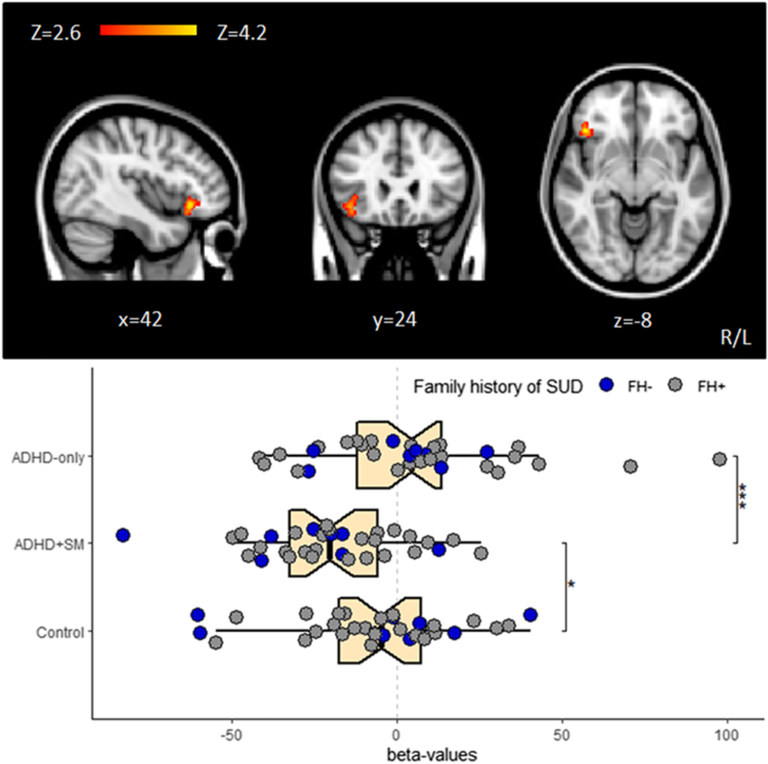
TABLE 1. Demographics and psychometric scores HCU (mean) SD Min-max HC (mean) SD Min-max Statistic p Effect sizec Age (years) 23.13 3.00 19–28 24.81 3.45 18–29 1.6425a 0.108 0.26 BDI 6.79 7.82 0–28 2.44 3.12 0–10 274.5b 0.022 −0.36 HAMD 1.33 1.88 0–8 0.44 0.81 0.2 251b 0.070 −0.29 Years of education 14.15 2.93 9–19.5 16.34 2.86 12–20 2.3464a 0.024 0.36 ADHD-SB total 11.5 5.88 2–23 8.19 8.92 0–26 259.5b 0.063 −0.29 Tobacco per year (pack years) 3.33 5.71 0–25.5 1.25 5.00 0–20 301b <0.001 −0.53 Joints lifetime 3731.25 4553.59 350–18 000 1.625 2.9 0–10 384b <0.001 −0.85 CUDIT total 17.63 8.88 4–36 0 0 0–0 384b <0.001 −0.86 Onset age 17.73 3.04 11–25 0 0 0–0 384b <0.001 −0.87 Duration use (years) 4.56 3.73 1–14.5 0 0 0–0 384b <0.001 −0.87 Current use (d/week) 5.65 1.67 2–7 0 0 0–0 384b <0.0011 −0.88 Current use (g/week) 6.06 6.39 0.25–28 0 0 0–0 384b <0.001 −0.86 Note: Significant results (pFDR < 0.05) in bold font. Abbreviations: ADHD-SB, attention-deficit/hyperactivity disorder self rating scale; BDI, Beck Depression Inventory; CUDIT, Cannabis Use Disorder Identification Test; HAMD, Hamilton Depression Scale; HC, control group (n = 16); HCU, heavy cannabis users (n = 24); SD, standard deviation; STAI, State–Trait Anxiety Inventory. a t value. b Wilcoxon rank-sum test value. 3.2 Parallel ICA

In the first step, component pre-selection identified two components, that is, one GMV- (p = 0.01) and one ALFF-component (p = 0.06). ANCOVA models revealed differences between HCU and HC in both GMV (F = 6.96, df = 1, p = 0.01) and ALFF (F = 5.00, df = 1, p = 0.03) component loadings. The spatial pattern for GMV comprised limbic-, thalamic-, cerebellar-, temporo-parietal- and temporo-occipital structures. For ALFF, the component pattern included occipital-, cerebellar-, frontal- and parietal structures (see Table 2 and Figure 1). The GMV component survived Bonferroni correction (p < 0.025), whereas the ALFF component did not. Nevertheless, given that several studies so far consistently highlighted the importance of prefrontal cortical function in substance-use disorders,55, 56 and cannabis-use disorders in particular,29, 57 the ALFF component was also considered for subsequent MRI-nuclear imaging cross-modal correlation analyses.

TABLE 2. Spatial characteristics of identified components of interest Component Brodmann area L R Volume (cc) L/R Region z-Score/MNI (x, y, z) z-Score/MNI (x, y, z) GMV Parahippocampal Gyrus 28, 34 6.5 (−23, −6, −20) 6.0 (23, −5, −20) 0.8/1.0 Thalamus - 5.9 (−8, −18, 11) 5.7 (8, −18, 11) 0.8/0.8 Uncus - 5.5 (−23, −3, −23) 5.3 (23, −2, −23) 0.4/0.3 Declive - 4.4 (−21, −65, −18) 5.1 (21, −77, −23) 0.5/1.5 Anterior Cingulate 24, 33 - 4.8 (3, 24, 24) −/0.5 Cingulate Gyrus 23, 24, 31, 32 4.0 (−2, −32, 33) 4.7 (3, 17, 30) 0.4/0.8 Supramarginal Gyrus 40 - 4.7 (53, −42, 35) −/0.4 Fusiform Gyrus 19 - 4.6 (24, −80, −21) −/0.4 INA Lingual Gyrus 17, 18 - 6.7 (9, −96, −21) −/0.3 Declive - - 6.2 (15, −90, −27) −/0.4 Middle Frontal Gyrus 6, 10, 11, 47 6.0 (−33, −6, 60) - 2.0/− Superior Frontal Gyrus 6, 8, 9, 10, 11 4.1 (−6, 6, 66) 5.3 (27, 66, −6) 0.4/1.1 Superior Parietal Lobule 7 4.8 (−36, −60, 57) 5.1 (30, −72, 51) 0.3/0.6 Precuneus 7 - 4.6 (24, −72, 51) −/0.3 Inferior Parietal Lobule 40 4.5 (−45, −48, 57) - 0.3/− Note: Voxels with z > 3.5 were coupled with the Talairach Daemon database to provide anatomical labels and were translated into MNI space. For each hemisphere (L = left; R = right), the maximum z-value and MNI coordinate are provided. The volume of voxels in each area is provided in cubic centimetres (cc); the table displays clusters >0.2 cc. Visualization of component patterns and loadings. (A) Left: overlays of the component pattern of GMV onto a brain template (axial slices). Right: boxplot of component loadings by group (p = 0.01; ANCOVA, adjusted for age). (B) Left: overlays of the component pattern of INA onto a brain template (axial slices). Right: boxplot of component loadings by group (p = 0.03; ANCOVA, adjusted for age). Please note that for the ALFF component, differences between HCU and HC did not survive Bonferroni correction for multiple comparisons (see also main test, Section 3). Colour bars depict z-values. HC, control group; HCU, heavy cannabis use group 3.3 Associations between component loadings and using behavior and prediction of current use

As expected, using behavior was highly intercorrelated (all Spearman's ρ's > 0.7). All loading component-using behavior pairing were significantly correlated (all Spearman's |ρ| > 0.30, all pFDR's < 0.05; generally, INA was stronger correlated than GMV), except lifetime number of joints and GMV, as well as CUDIT and GMV. GMV and INA were not intercorrelated (see Figure 2 and Table S1).

Correlograms between component loadings and using behavior. The shape of the ellipse represents the extent of the correlation between two variables, more circular when two variables are uncorrelated. The slope of the longest axis of the ellipse indicates the direction of the correlation, with a positive slope indicating a positive correlation. Black background highlights correlations surviving p < 0.05 FDR-correction. Note that for display purposes, no background-highlighting was done for using behavior intercorrelations. Colour bar depicts Spearman's ρ

Regression models revealed lifetime use to be the best predictor for current use, whereas amount of current use could be predicted better than frequency of current use (see Table 3 for details). The best performing model (in terms of best adjusted R2 following Stein's formula58 and using minimum amount of predictors) predicted amount of current use using number of lifetime joints and GMV component loadings as predictors (adjusted R2 = 0.59, p < 0.00001). MRI-nuclear imaging cross-modal correlations between affected receptor systems and pICA components.

TABLE 3. Prediction of current use via lifetime use and/or component loadings Measure of current use Predictors Multiple R2 Adjusted R2 (Stein) p model D/week Joints lifetime 0.28 0.22 0.0004548 GMV 0.19 0.12 0.005556 ALFF 0.1 0.03 0.04827 Joints lifetime, GMV 0.39 0.3 0.000107 Joints lifetime, ALFF 0.36 0.27 0.0002785 GMV, ALFF 0.25 0.15 0.00468 Joints lifetime, GMV, ALFF 0.45 0.33 0.00007825 G/week Joints lifetime 0.57 0.53 <0.00001 GMV 0.17 0.11 0.007711 ALFF