1 INTRODUCTION

Oil palm plantations (dominated by plantings of the African oil palm Elaeis guineensis Jacq.) covered over 18.7 million hectares (Mha) worldwide in 2017 and continue to increase (Meijaard et al., 2018). Much of this expansion has been in Borneo where at least 3.06 Mha of species-rich old-growth forests were converted to industrial plantations between 2000 and 2017 (Gaveau et al., 2018). Such dramatic changes in land cover have major ecological consequences, highlighting the need for research that contributes to the healthy functioning of this important and widespread landscape (Foster et al., 2011). Seeking the best ways to maintain ecological complexity by incorporating forest and other vegetation has become an important issue for plantation owners and planners (Meijaard et al., 2016; Yahya et al., 2017). One motivation for this is to maintain a range of different taxa, including wild pollinators, within the landscape.

Although pollinators are mobile, they can be greatly affected by habitat fragmentation. The conversion of native forests to cultivated land has the potential to cause the loss of both feeding sites (sources of pollen and nectar) and suitable nesting habitat for pollinators (Patrício-Roberto & Campos, 2014). The habitat requirements of pollinators can be complex (e.g., different nesting and foraging habitats; Antoine & Forrest, 2020; Westrich, 1996), which makes them particularly sensitive to habitat loss and fragmentation. Most (an estimated 94%) tropical flowering plants are animal-pollinated (Ollerton et al., 2011). A decline in pollinators thus impacts the reproduction of wild plants and consequently entire ecosystems (Burkle et al., 2013; IPBES, 2016; Potts et al., 2010). Landscape changes, including those within the remnant fragmented areas, may cause loss of genetic variability and population stability, potentially leading to the disappearance of populations (Patrício-Roberto & Campos, 2014; Sodhi et al., 2004) and having severe effects on pollinator services (Potts et al., 2010).

Many food crops require animal pollination to maximize fruit set, size, and quality (Ollerton et al., 2011). Even oil palm is primarily pollinated by African weevils (Elaeidobius kamerunicus Faust) that increase fruit set and yield (Caudwell, 2001; Zulkefli et al., 2021). Wild pollinators in particular contribute to the productivity and viability of many crops (Garibaldi et al., 2013) and thus to food security and nutrition (Ellis et al., 2015; Garibaldi et al., 2016). Evidence of this exists for many crops including watermelon (Sawe et al., 2020), tomatoes (Cooley & Vallejo-Marin, 2021; Neto et al., 2013), and chilies (Landaverde et al., 2017). Land-use conversion can disrupt pollination services on which the crops depend (see, e.g., Klein et al., 2003; Ricketts et al., 2008). Such disruptions add to the pollinator declines already seen worldwide, reflecting not just habitat loss but also damaging land-use practices (e.g., pesticide use) and climate change (Potts et al., 2010). While oil palm has raised incomes and living standards in Indonesia (Qaim et al., 2020), there are concerns that diet quality may have declined (Food Security Council et al., 2015; Ickowitz et al., 2016). One possible reason is the difficulty of producing highly nutritional, pollination-dependent food crops in landscapes with insufficient pollination services.

We recognized that a better understanding of pollinator activity may contribute to improved planning and management of the landscape to maintain local pollinators and their beneficial role. Here, we assess bee activity within a landscape of industrial oil palm and remnant forest in West Kalimantan, Indonesia. Our main aim was to determine whether the number of bee visits to flowers is affected by distance to forest. We hypothesize that the frequency of bee visits to flowers of the selected plant species will decrease with distance from forest. A further aim of our study was to test whether flower visitation rates by bees were dependent on the distance to the nearest planted oil palm patch. We expect palm trees to have conditions more similar to forest and to provide more resources for bees than agricultural fields, fallows, and other open land. Therefore, we hypothesize there will be an increase in bee visits when flowers are closer to planted palm compared with non-forested areas. To answer our study questions, we observed bee visits to six plant species and related the visitation frequencies to distance from forest while controlling for weather and time of day. To our knowledge, this is the first study to assess bee visitation frequency to both wild plants and food crops within an oil palm-dominated landscape.

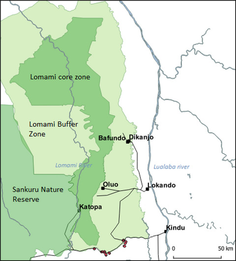
2 METHODS 2.1 Study area

This study was conducted from June to November 2017 within the concession of PT Kayung Agro Lestari (KAL) in Kabupaten Ketapang in the province of West Kalimantan, Borneo, Indonesia (1°26′00.0″S 110°13′00.0″E; Figure 1a). The plantation is owned and managed by PT Austindo Nusantara Jaya (ANJ), a member of the Roundtable on Sustainable Palm Oil (RSPO) (PT Austindo Nusantara Jaya Tbk, 2016). Before conversion to oil palm plantation, the landscape was primarily logged-over natural forest (~8600 ha) and degraded land (Meijaard et al., 2016). Conversion started in 2010 and by 2016, 12,061 ha out of the 17,998 ha had been planted (Meijaard et al., 2016; PT Austindo Nusantara Jaya Tbk, 2016). Here, we use the terms “oil palm plantation” and “plantation” when referring to the entire area inside of the concession and “planted oil palm” when referring to sections of monoculture planted oil palm within the plantation.

(a) Location of the study area on the West coast of Indonesian Borneo. (b) Setup of a Brinno BCC200 Pro camera using a T1 Clamp tripod attached to a wooden pole, to observe planted Turnera subulata adjacent to oil palm. (c) An image captured by a Brinno BCC200 Pro camera of a bee visiting a T. subulata flower

The majority of the planted oil palm grows on shallow peat (~63%), with less on mineral soil (~33%) and sands (~4%). The palms are planted about 9 m apart resulting in a mostly closed canopy. Intensive maintenance, including regular physical clearance of ground vegetation and application of herbicides, results in little understory vegetation among the planted palms. Sixteen forested areas (20–2333 ha), 21% (3884 ha) of the concession, have been identified as having High Conservation Value (HCV) and are regularly monitored by the company (Meijaard et al., 2016).

2.2 Study species

We studied bee visits to six angiosperm species (Table S1). Four of these (Capsicum frutescens L. “chili,” Citrullus lanatus (Thunb.) Matsum & Nakai “watermelon,” Solanum lycopersicum L. “tomato,” and Solanum melongena L. “eggplant”) are common local crops. The other two, the native Melastoma malabathricum L. and the introduced Turnera subulata Smith, have a wide distribution throughout the plantation. All the focal species are non-native except M. malabathricum, which is a common colonizing plant that occurs in cleared, degraded areas near forest edges within the plantation. T. subulata is planted as a method of bio-control for leaf-eating caterpillars (fire- and bagworms), common pests to oil palm (Rashid et al., 2014).

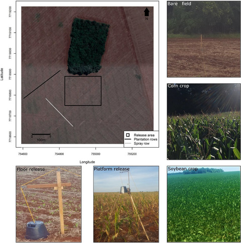
2.3 Study design

We conducted two studies: The first (hereafter referred to as the “Grid Study”) was a systematically planned study of crop plants within an extensively cleared area of several hectares and the second was a transect study (hereafter referred to as the “Transect Study”). The Grid Study spanned up to a maximum distance of 208 m from forest and 144 m from planted palm (Figure 2a), while the Transect Study spanned from the forest edge up to 2130 m from natural forest.

(a) Schematic (not to scale) of the grid layout of the crop plant plots for the Grid Study. The observed plants were the crop species (Citrullus lanatus, Solanum melongena, Capsicum frutescens, and Solanum lycopersicum), as well as some Solanum malabathricum and Turnera subulata growing at the study site. (b) Schematic (not to scale) of the transect layout for Transects A, B, C, D, E, and F in the Transect Study. The figure shows one representative transect. T. subulata was the only observed plant species

Transect locations were chosen to represent a range of forest sizes and distances from these (Table S2). Forest 1 is a large, continuous forest that extends beyond the plantation boundary; Forest 2 is a conserved forest within the plantation that extends beyond the boundary; and Forest 3 is an isolated secondary forest hill surrounded by oil palm. The Grid Study was conducted in relation to Forest 4, an isolated hill that has been classified as a high conservation value area.

2.3.1 Grid Study

We conducted the Grid Study between 22 July and 5 September 2017. In total, we obtained 397 plants, growing in individual poly bags. Due to mortality at the nursery, the number of individuals varied among the species: 134 C. lanatus, 108 S. melongena, 105 S. lycopersicum, and 50 C. frutescens. We placed the nursery-grown plants in a grid consisting of twelve plots, with three columns following a gradient from edge of forest and four rows following a gradient from edge of planted oil palm. Each plot had about six columns and six rows of plants, with ~0.5 m spacing between the plants. Plants were assigned randomly to ensure each plot consisted of a representative sample of all study species. The area already had scattered individuals of naturally growing M. malabathricum and planted T. subulata, allowing assessment of the effect of distance to forest and to planted palm using all six study species.

2.3.2 Transect Study

We conducted the Transect Study from 15 to 29 October 2017. We observed visits to one plant species, T. subulata, within six different transects (Transects A–F). Transects were established in relation to three forested areas (Figure 2b), with each forest having two transects adjacent to it (Figure S1). The transects were located along roadsides where T. subulata had been planted, starting as close to the forest edge as possible and continuing for at least 300 m into planted oil palm. Along each transect, we identified four observation points. The T. subulata growing closest to the edge of forest was designated as observation point one. We then walked along the transect for about 100 m, measured by a handheld GPS unit, where we located the closest T. subulata bush as the second observation point. This process was then repeated for the remaining two observation points. The observation points were selected based on the presence of at least one T. subulata bush. The distance between observation points, and the maximum distance from forest (Table S3), varied due to the variation in spacing between the planted T. subulata. To assess pollinator activity further within planted oil palm, we established four additional observation points located more than 800 m from the forest (with a range from 824 to 2130 m) (Figure S1). Final distances between each observation point and the edge of the nearest forest, observed from satellite imagery, were measured using Google Earth.

2.4 Data collection for both Grid and Transect Studies 2.4.1 Direct flower visit observations

To estimate flower visitation frequencies, we observed pollinator visits to flowers on all the above-mentioned plant species. We define a visit as a pollinator making apparent contact with the stigma or anthers of the preselected flowers. Each observation period lasted 10 min, and all were conducted by the same observer. During the observation period, all observed pollinator visits were recorded, but later we focused on analyzing only the bee data. Due to taxonomic challenges and the low numbers of visits from some morpho-species, we analyzed all bees as one group. Specimens in an adjacent study were collected and photographed (Hessen, 2020), and visual identification of these specimens was carried out by John S. Ascher based on diagnostic characters documented in Soh and Ascher (2020).

The number of observed flowers for each observation varied, depending on how many flowers were open and their aggregation (ensuring the observer, or the camera, could adequately monitor all flowers simultaneously; range: 1–36, mean: 4.6). The sequence and starting point of which the transects, and plots along the transects, were observed was chosen at random. Observations were conducted between 05:30 and 18:00 h (mean: 1000 h), with most being during morning hours when most flowers were open. Observations were not conducted during rain.

2.4.2 Flower visit observations with cameras

We used Brinno BCC200 Pro cameras to perform additional flower visit observations. We used a T1 Clamp tripod to attach the camera to a wooden pole that would stand vertically when placed into the ground (Figure 1b). We adjusted the focus of the cameras manually during each setup. The cameras were set to have a frame rate of one picture per second and with a resolution of 1280 × 720 pixels (Figure 1c). The individual recordings lasted longer than 10 min, but to keep the observations comparable with the direct observations, we treated every 10 min as a separate observation. To count the number of flower visits recorded with the camera, we later viewed the videos on a computer using the Brinno Video Player. Camera observations were conducted in both studies and took place on the same observation days as the direct observations. The percentage of observations conducted with the cameras varied per transect from 0% to 60% (Table S3). The photographs did not allow for identification of pollinators below order level.

2.4.3 Environmental variables

For each observation period, we recorded time of day, temperature, and relative humidity with a Suncare thermo-hydrometer (model 303C). We subjectively categorized wind, wetness of the vegetation, and sun exposure (Table S4). We also obtained data on daily rainfall from a weather station at the plantation, and we used a weather logger (UA-002 HOBO) placed at a fixed point within the plantation to record light intensity and air temperature at 3-hour intervals. We obtained additional weather data from a meteorological station in Ketapang (~50 km from the study site) and in Pontianak (~188 km from the study site; Table S4).

In the Grid Study, the mean temperature of the observation periods was 28.8°C (23.8–34.0°C) and the mean humidity was 72.4% (50%–96%). In the Transect Study, the mean temperature of the observation periods was 28.5°C (25–32.4°C) and the mean humidity was 79.4% (60%–94%).

2.5 Statistical analyses 2.5.1 Variables

We collected data on various factors that might influence pollinator activity. We placed the variables into five categories: weather (including temperature, humidity, precipitation, and sunlight), temporal (including time of day and day of year), environmental (including forest ID, size of forest, and soil type), spatial (including distance from forest and distance from oil palm), and observed plant (including plant species, number of flowers observed per observation, recording ID and observation method). See Table S4 for more details on all of the variables we identified.

2.5.2 Analyses

All data analyses were performed using R (version 3.5.1 with macOS version 10.14.6; R Core Team, 2018). We conducted initial data exploration following Zuur et al. (2010) on all variables (Table S4). To analyze the relationship between flower visitation frequencies and a number of explanatory variables, we generated generalized linear mixed models (GLMMs) with a Poisson error (log link) distribution. Number of visits was used as the response variable and the number of flowers observed was included as an offset variable in all models, following Reitan and Nielsen (2016). Observation ID was included in each model as a random effect to account for overdispersion (Harrison, 2014). Other variables considered as random effects include transect, plot, day, and recording ID. All models were generated using the “glmer” function in the R package “lme4” version 1.1-15 (Bates et al., 2015) with the “bobyqa” optimizer. Continuous variables were centered and scaled using the “scale” function (R Core Team, 2018). We used an information-theoretic approach to identify the most parsimonious model using the Bayesian information criterion (BIC). Variance inflation factors (VIFs) were assessed using the “vif” function in the R package “car” (Fox & Weisberg, 2011). Dispersion, zero-inflation, and uniformity were tested using "testDispersion," “testZeroInflation,” and “testUniformity” functions in the R package “DHARMa” version 0.3.2.0 (Hartig, 2020). Confidence intervals were calculated using the Wald method with the “confint.merMod” in the R package “lme4” version 1.1-15 (Bates et al., 2015). Pseudo R2 values (delta method) were generated for each model using the “r.squaredGLMM” function in the R package “MuMIn” version 1.42.1 (Bartoń, 2018). Figures 3 and 4 were created using “ggplot” function in the R package “ggplot2” version 3.3.2 (Wickham, 2016). Effect of predictors for each model was generated using “allEffects” function in the R package “effects” version 4.1.0 (Fox, 2003, 2019).

(a) Expected visitation frequency per flower per 10-min observation period in the Grid Study in relation to distance from forest (m), with all other variables remaining constant. Expected visitation frequencies are based on Model 1 estimates, and shaded area represents upper and lower estimates (n = 667). (b) Bee visits per flower per 10-min observation period in the Grid Study, in relation to distance from forest (m). Points represent raw observed bee visits per flower per 10-min observation period (n = 723). (c) Expected visitation frequency per flower per 10-min observation period to each study species, with all other variables remaining constant. Points represent Model 1 estimates, and error bars represent upper and lower estimates (Melastoma malabathricum n = 32, Turnera subulata n = 75, Solanum melongena n = 94, Citrullus lanatus n = 186, and Capsicum frutescens n = 280)

(a) Expected visitation frequency per flower per 10-min observation period in the Transect Study in relation to distance from forest (m), with all other variables remaining constant. Expected visitation frequencies are based on Model 2.1 estimates, and shaded area represents upper and lower estimates (n = 301). (b) Bee visits per flower per 10-min observation period in the Transect Study, in relation to distance from forest (m). Points represent raw observed bee visits per flower per 10-min observation period (n = 301). (c) Expected visitation frequency per flower per 10-min observation period to Turnera subulata adjacent to the three study forests in the Transect Study, with all other variables remaining constant. Points represent Model 1.2 estimates, and error bars represent upper and lower estimates (Forest 1 n = 96, Forest 2 n = 125, and Forest 3 n = 80). (d) Expected visitation frequency per flower per 10-min observation period to T. subulata <450 m from forest and >800 m from forest in the Transect Study, with all other variables remaining constant. Points represent Model 2.2 estimates, and error bars represent upper and lower estimates (<450 m n = 301, >800 m n = 22)

3 RESULTS

The field observations revealed a diversity of flower-visiting insects with bees, the most frequently observed visitor to all species, making up 81.4% of the total number of observed visits (Figure S2a,b). Specimens collected in an adjacent study (Hessen, 2020) show that pollinators in the study site included individuals of the following genera: Apis sp., Ceratina sp., Geniotrigona sp., Heterotrigona sp., Homotrigona sp., Lasioglossum spp., Lipotriches sp., Nomia spp., and Xylocopa spp..

In the Grid Study, we counted 355 bee visits to 2071 flowers during 723 10-min observation periods over 32 days. The mean visits per flower for all plant species combined was 0.23 per 10-min period (0.19 when observed manually and 0.31 when recorded by the cameras [Table 1]). In the Transect Study, we counted 894 bee visits to 2760 flowers during 323 10-min observation periods over 15 days. The overall mean visits per flower were 0.34 per 10-min observation (0.52 when observed manually and 0.16 when recorded by cameras [Table 1]).

TABLE 1. Summary of bee visits in both studies during 1046 observation periods between 22 July and 29 October 2017 Species # Of visits observed # Of observation periods # Of observation days Range of observation dates (dd/mm) % Of observation periods with zero visits Max visits/flower/10 min Mean visits/flower/10 min Study Citrullus lanatus 184 186 25 24/07–05/09 64.5 7 0.62 1 Turnera subulata 89 75 5 22/07–28/07 53.3 2.0 0.33 1 Melastoma malabathricum 30 32 13 25/07–05/09 78.1 2.5 0.19 1 Solanum melongena 42 94 19 28/07–05/09 85.1 3.5 0.18 1 Capsicum frutescens 10 280 24 28/07–05/09 98.6 1.5 0.01 1 Solanum lycopersicum 0 56 21 30/07–05/09 100 0 0 1 T. subulata 894 323 15 15/10–29/10 39.0 6.3 0.34 2 Note # of visits observed = total number of bee visits in all 10-min observation periods combined. Study 1 = small-scale grid-based study (Grid Study), Study 2 = large-scale transect study (Transect Study).

As we recorded no visits to S. lycopersicum flowers (n = 56 observation periods), we excluded this species from further analyses. The flower visits recorded in the two studies were analyzed separately.

3.1 Factors explaining variation in visit frequency in the Grid Study

Our best model (Model 1) explaining how visitation frequency to flowers varied in the Grid Study (R2m = 0.520, R2c = 0.947) included distance from forest, plant species, sun, time of day, and sampling method (camera or manual observation) as fixed effects (Table 2). The estimated relative contribution of explained variation for each variable in the model is listed in Table S5a. The estimated effect of each predictor (based on Model 1) with all other variables being held constant is listed in Table S6a. VIF for each variable is <2.

TABLE 2. Output for the GLMM (Model 1) that best explains the variation in bee visit frequency to flowers in the Grid Study, based on 667 observation periods Fixed effect Estimate SE 95% Confidence limits p-Value Lower Upper Intercept −6.16 0.485 −7.11 −5.21 <0.001 Forest distance −0.270 0.134 −0.533 −0.00605 <0.05 Camera (yes) 0.739 0.304 0.143 1.33 <0.05 Species (Melastoma malabathricum) 2.37 0.663 1.07 3.67 <0.001 Species (Solanum melongena) 2.99 0.529 1.95 4.03 <0.001 Species (Turnera subulata) 2.77 0.518 −1.76 3.79 <0.001 Species (Citrullus lanatus) 3.68 0.478 2.74 4.61 <0.001 Time of day −0.397 0.176 −0.741 −0.0525 <0.05 Sun (some) 0.712 0.292 0.141 1.28 <0.05 Sun (yes) 1.17 0.365 0.456 1.89 <0.01 Note All continuous variables were centered and scaled. Forest Distance = Distance (m) from nearest forest. Camera = Whether observation was observed in field or via camera (factor, 2 levels: yes, no). Species = Plant species observed (factor, 5 levels: C. lanatus, T. subulata, M. malabathricum, S. melongena, and C. frutescens). Time of day = Minute of the day observation was started. Sun = Presence of direct sunlight on observed flowers (factor, 3 levels: yes, some, no). SE = standard error. Confidence intervals calculated using Wald method. The random effect is “observation ID” (n = 667).

There was a significant decrease in visitation frequency with greater distance from forest (Figure 3a), with the expected visitation frequency decreasing by 55.4% at the maximum distance of 208 m from forest. We did not detect any influence of distance from oil palm on visitation frequency. There was variation in visitation frequency among the focal plant species. C. lanatus had the highest visit frequency, followed by T. subulata, S. melongena, M. malabathricum, and C. frutescens (Figure 3b,c). Expected visitation frequency was positively associated with observed flowers being in direct sunlight. Time of day also showed a positive linear association with visit frequency. Temperature and humidity were highly correlated with time of day, and thus, we were unable to disentangle the effects of these three variables. Therefore, although we expect temperature and humidity to play an important role, they were not included in the best model. We did not anticipate the observation method would influence the number of observed visits. However, analyses showed that the cameras revealed a higher visit frequency than human observations.

3.2 Factors explaining variation in visit frequency in the Transect Study

We developed two models to describe how visit frequency to T. subulata varied in the Transect Study. The first model (Model 2.1) included observation points spanning from the forest edge to 483 m into planted oil palm (and did not include observation points >800 m from forest; R2m = 0.270, R2c = 0.445), while the second model (Model 2.2) included data from all observation points as a 2-level fixed factor discriminating between plots situated <450 m or >800 m from forest (R2m = 0.259, R2c = 0.451). The estimated relative contribution of explained variation for each variable in each models is listed in Table S5b,c. The estimated effect of each predictor (based on Model 2.1 and 2.2) with all other variables being held constant is listed in Table S6b,c. VIF for each variable is <2.

Model 2.1 included distance from forest, forest ID, sun, time of day, and camera as fixed effects (Table 3). We found a significant decrease in visitation frequency with an increase in distance from forest (Figure 4a). The expected visitation frequency decreased by 52.6% at the maximum distance from forest of 438 m. The best model included forest ID showing that the larger forests (Forests 1 and 2) had similar and higher visitation frequencies compared with the smaller forest (Forest 3; Figure 4b). The expected visit frequency for Forest 3 at any distance was 70.3%–76.5% lower than for Forests 1 and 2, respectively (Figure 4c). Visitation frequency was positively associated with direct sunlight. Time of day had a negative linear relationship with visit frequency, and camera observations unexpectedly had significantly lower observed visitation frequencies.

TABLE 3. Output for the GLMM (Model 2.1) that best explains the variation in bee visit frequency to Turnera subulata in the Transect Study based on 301 observation periods Fixed effect Estimate SE 95% Confidence limits p-Value Lower Upper Intercept −2.18 0.324 −2.81 −1.54 <0.001 Forest distance −0.249 0.0788 −0.403 −0.0943 <0.01 Forest 2 0.232 0.167 −0.0951 0.559 0.165 Forest 3 −1.21 0.215 −1.64 −0.793 <0.001 Sun (some) 1.37 0.308 0.768 1.98 <0.001 Sun (yes) 1.83 0.326 1.19 2.47 <0.001 Time of day −0.209 0.0824 −0.371 −0.0479 <0.05 Camera (yes) −1.59 0.155 −1.89 −1.29 <0.001 Note All continuous variables were centered and scaled. Forest Distance = Distance (m) from nearest forest. Forest = The closest forest (factor, 3 levels: 1, 2, and 3). Sun = Presence of direct sunlight on observed flowers (factor, 3 levels: yes, some, no). Time of day = Minute of the day observation was started. Camera = Whether observation was observed in field or via camera (factor, 2 levels: yes, no). Confidence intervals calculated using Wald method. SE = standard error. Random effect is “observation ID” (n = 301).

Model 2.2 included distance from forest (as a factor: <450 m or >800 m from forest), forest ID, sun, time of day, and camera as fixed effects. Visitation frequencies were significantly higher near forests, with expected visitation frequency being 66.2% lower at distances greater than 800m from the forest edge than at distances less than 450 m (Figure 4d). The other fixed effects showed similar patterns as for Model 2.1 (Table 4).

TABLE 4. Output for the GLMM (Model 2.2) that best explains the variation in bee visit frequency on Turnera subulata