Cell reprogramming

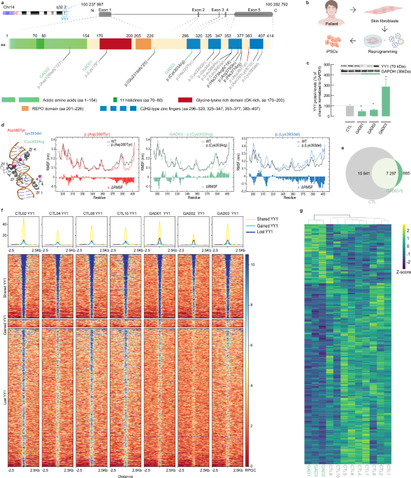
Human fibroblasts were isolated from skin biopsies and lymphoblastoid cell lines (LCLs) were generated by Epstein-Barr virus (EBV) transformation of the B-lymphocytes within the peripheral blood lymphocyte leading to proliferation and subsequent immortalization of these cells. Both non affected and affected individual’s - samples (fibroblasts and LCLs) were reprogrammed using the non-integrating Sendai virus (SeV) method to safely and efficiently deliver and express key genetic factors (Yamanaka factors OCT3/4, SOX2, KLF4, and c-MYC). For all lines, a total of 3 × 105 cells were transduced per individual using a multiplicity of infection (MOI) of 5-5-3 (KOS comprising human Klf4, Oct3/4, and Sox2; c-MYC containing human c-Myc; Klf4 with human Klf4, respectively). Moreover, the amount of virus used was calculated according to each certificate of analysis respective of each SeV kit. The reprogramming procedure was performed according to the manufacturer’s protocol using feeder-dependent protocols for both fibroblasts and PBMCs (feeder layer containing mouse embryonic fibroblasts). Cells were maintained every day and small colonies were subsequently picked and expanded approximately 1–1.5 months post-transduction. After reprogramming from LCL, EBV expression in iPSCs was evaluated, and samples completely turned off EBV expression compared to a positive control cDNA taken from LCL, showing irrelevant Ct, and with melting curves comparable with the negative (no cDNA). Reprogrammed fibroblast-derived iPSCs were also validated to be free of SeV transduced vectors by RT-qPCR. iPS cells were pulled down and pelleted for RNA extraction and depletion was checked by RT-qPCR according to manufacturer’s instructions. A reverse transcription was carried out using 2.5 μg of RNA following the instructions provided with the kit (Cat N°, 11766050, Invitrogen). For PCR reaction mix preparation, 12 ng of cDNA for each sample was used and performed in triplicates using the Fast SYBR Green Master Mix (visualize primers in Table S2). Positive control cells were set aside during the first stages of the reprogramming procedures (Fig. S1, Cat N° A16517, ThermoFisher).

Cell cultureFibroblast/LCL handling and iPSC culturing

Human fibroblasts were cultured in DMEM, FBS 10%, non-essential amino acids (NEAA) 1%, penicillin-streptomycin (P/S) 1%, and β-mercaptoethanol 0.1%. LCLs were grown in RPMI 1640, FBS 15%, HEPES 1%, L-glutamine (Gln) 1%, and P/S 1%. Trypsin was used to passage fibroblasts whereas LCLs were cultivated in suspension and expanded by dilution. Human iPSCs were cultured in feeder-free conditions onto matrigel-coated dishes using TeSR-E8 medium supplemented with P/S 1% and passaged using either ReLeSR (Cat N° 100-0483 stemcell technologies, generates cell aggregates for expansion and standard maintenance) or Accutase solution (Cat N° A6964 Sigma, exclusively for experimental procedures) supplemented with ROCK inhibitor 5 μM (Y-27632 dihydrochloride, #A3008 ApexBio) was added to the culture to enhance single cell survival. Cryopreservation of hiPSCs was performed in complete TeSR-E8 medium with 10% DMSO and supplemented with ROCK inhibitor 5 μM. All samples were routinely tested for mycoplasma.

Directed differentiation of hiPSCs into ectoderm, mesoderm, and endoderm lineages

To functionally validate the potential of human iPSC lines to differentiate into all three embryonic germ layers, we took advantage of the STEMdiffTM trilineage differentiation Kit and followed the manufacturer’s instructions with minor modifications (Cat N° 05230, Stemcell technologies). hiPSCs were cultured onto Matrigel-coated glass coverslips and on day 0, 2.5 × 105, 7.5 × 104 and 2.5 × 105 cells were plated for further differentiation into ecto-, meso-, and endoderm, respectively. At the end of differentiation, cells were fixed, and lineage-specific markers were used for immunofluorescence using the following established markers NESTIN and PAX6 for ectoderm; Brachyury and CXCR4 for mesoderm; and FOXA2 and SOX17 for endoderm (Fig. S2).

Differentiation of iPSCs into neural crest stem cells (NCSCs)

hiPSCs were differentiated into NCSCs as previously described [62]. NCSC differentiation required 15–20 days and was carried out as follows: 90% confluent iPSCs were detached with Accutase solution and plated onto matrigel-coated dishes using TeSR-E8 medium supplemented with 5 μM ROCK inhibitor at a density of approximately 9.2 × 104 cells per cm2. After 24 h, NCSC differentiation medium was added and changed every day. NCSC medium was composed of DMEM-F-12 1:1, 10% probumin (stock solution of 20% m/v in DMEM F-12 1:1), P/S 1%, L-Glutamine 1%, NEAA 1%, trace elements complex 0.1, 0.2% β-mercaptoethanol (50 mM), Transferrin (10 μg/mL), sodium L-ascorbate (50 μg/mL), Heregulin-1 (10 ng/mL), LONG®R3 IGF-I (200 ng/mL), FGF2 (8 ng/mL), GSK3 inhibitor IX Bio (3 μM) and SB431542 (20 μM). Cells were passaged every 4–5 days and plated at high densities. Upon differentiation, NCSC were stocked as stable lines and cultured using NCSC medium with routine splitting ratios of 1:4–5 (Fig. S3e, f).

Preparation of primary mouse astrocytes

Primary astrocyte cultures were created from the cerebral cortices of embryonic day 18 (E18) mice embryos and maintained as previously described [63, 64]. In a nutshell, after embryo collection, cortices were dissected from each embryo’s brain, and chemical dissociation with trypsin (2.5%, at 37 °C for 30 min) was performed. Afterwards, mechanical dissociation was performed by vigorous pipetting. Following digestion, cortex tissues were centrifuged (300 g for 5 min) and supernatant discarded. Finally, astrocyte medium (DMEM supplemented with DMEM medium supplemented with FBS 20%, P/S 1%) was added and 1–1.5 × 107 cells were seeded in each T75 culture flask. After reaching confluence (10–15 days), astrocytes were passaged with trypsin and expanded. This protocol allowed the generation of pure astrocytic cultures due to the gradual absence of viable neurons and other glial cells. Astrocytes were generated and maintained 3–4 weeks prior NGN2-derived neuron differentiation.

Differentiation of iPSCs into NGN2-derived cortical neurons

hiPSCs were engineered using a ePiggyBac (ePB) transposon previously electroporated using the Neon™ Transfection System (MPK5000, ThermoFisher). Electroporation parameters for each reaction of 4 × 105 cells were: 900 V, 20 ms, 2 pulses using 5 μg of total DNA in a 1:10 ratio of helper:vector (0.5 μg of an helper plasmid expressing a transposase and 4.5 μg of donor plasmid with a transposable element). NGN2 ePB donor plasmid has the following genetic configuration: hUbC promoter - rtTA - T2A - BsdR - TRE - Ngn2 - P2A - EGFP - T2A – PuroR and allows the selection with blasticidin (Fig. S7a). Following transfection, cells were allowed to recover for 48 h and selection was performed using blasticidin 5 μg/mL until all cells were eliminated from the negative control performed without the addition of the transposase (usually 5–7 days of selection). Stable iPSCs containing the ePB transposon were stored until needed for neuronal differentiation.

Neuronal differentiation is induced by doxycycline and is followed by NGN2 overexpression, as previously described [65]. Cortical neurons were maintained in Neurobasal medium fully supplemented (B27 with vit.A + P/S + Glutamax + doxycycline + puromycin + N2 + NEAA + human Laminin + NT3 + BDNF). Fresh mouse astrocytes were added to the culture by means of hanging cell culture inserts (MCRP06H48, Millipore, transwell for clarity) on day 4 after definitive plating of neurons in poly-d-lysine-coated 6 well plates or added into poly-L-ornithine-coated glass coverslips treated with nitric acid for IF experiments at a ratio 1:1 (human neuron to mouse astrocyte).

Differentiation of iPSCs into 3D human in vitro systems – cortical brain organoids

Cortical brain organoids were generated using an adaptation of a previously described protocol [36]. Prior to organoid culture, iPSCs were instead routinely cultured with mTeSR™1 basal medium (Cat N° 85850 stemcell technologies). hiPSC were expanded in 10 cm dishes and detached at 60–70% confluency with Accutase solution for obtaining single cell suspensions. After centrifugation (150 g, 3 min), cells were resuspended in mTeSR™1 basal medium supplemented with ROCK inhibitor (5 μM), TGF-β inhibitor SB-431542 (10 μM), and dosromorphin (1 μM) and counted. To form free-floating spheres, approximately 4 × 106 cells were added to a single 6-well plate and kept under rotation (95 rpm) inside the incubator (37 °C, high O2 conditions) for 24 h. The medium was refreshed every day by removing half (2 mL) and adding half (2 mL) for the following 2 days. After 3 days (day 4 to 10), supplemented mTeSR™1 basal medium was replaced by Media 1, comprised of Neurobasal A medium supplemented with 1% GlutaMAX, 1% N2 NeuroPlex, 1% B27 with vitamin A, 1% NEAA, 1% P/S, SB (10 μM) and Dorsomorphin (1 μM). Subsequently, from days 11 to 17, cells were maintained in Media 2: Neurobasal A medium with GlutaMAX, 1% B27 + vitamin A, 1% NEAA and 1% P/S supplemented with FGF2 (20 ng/mL), followed by 7 additional days (day 18 to 24) in Media 2 supplemented with FGF2 (20 ng/mL) and EGF (20 ng/mL) to boost neural progenitor proliferation. Finally, organoid medium conditions shifted to Media 3, composed of Media 2 supplemented with BDNF (10 ng/mL), GDNF (10 ng/mL), NT-3 (10 ng/mL), L-ascorbic acid (200 μM) and dibutyryl-cAMP (1 mM) to promote network maturation, gliogenesis and enable neuronal activity. After 7 days (31 days in vitro), cortical organoids were maintained in Media 3 for as long as needed, with media changes every 3–4 days. Catalog numbers for all reagents and small molecules used for the cell culture medium were previously described [36].

RNA extraction and library preparation for bulk RNA sequencing (RNA-seq)

Cultured iPSCs and NGN2-derived neurons were washed with phosphate-buffered saline (PSB) and treated with 600 μL RTL buffer supplemented with 10% β-mercaptoethanol. Afterwards, total RNA was extracted using the RNeasy Mini Kit. Purified RNA was quantified using a NanoDrop spectrophotometer and RNA quality was further checked with an Agilent 2100 Bioanalyzer using the RNA nano kit (Cat N° 5067-1511, Agilent). Only samples with RIN > 9 were used for library preparation. Prior to library preparation, ERCC spike-in mixes (Cat N° 4456739, ThermoFisher) were added to all samples to facilitate data normalization and quantification. RNA sequencing libraries were prepared following manufacturer’s protocols for Truseq-stranded Total RNA (RiboZero depletion) or using Illumina Stranded mRNA Prep, starting from 250–500 ng of total RNA. cDNA library quality was assessed on Agilent 2100 Bioanalyzer, using the Agilent High Sensitivity DNA Kit (Cat N° 5067-4626, Agilent). Libraries were then sequenced with the Illumina Novaseq 6000 instrument at a read length of 50 bp (paired-end) with a coverage of 35 million reads per sample.

Chromatin immunoprecipitation followed by sequencing (ChIP-Seq)

ChIP-seq for TF YY1 was performed in all iPSC lines (4 CTLs vs. 3 GADEVS lines) using approximately 1 × 107 cells per sample. First, cells were harvested and crosslinked with formaldehyde 1% in PBS for 8 min at RT under continuous rotation. To quench the reaction, glycine (125 μM) was added to each mix and incubated for 5 min on ice. Cells were subsequently pelleted by centrifugation (500 g, 3 min at 4 °C) and washed in ice-cold PBS. Cells were lysed in 10 mL buffer A (50 mM HEPES pH 8.0, 140 mM NaCl, 1 mM EDTA, 10% glycerol, 0.5% NP-40, 0.25% Triton X-100) for 10 min on ice. After centrifugation, cell pellet was resuspended in 5 mL buffer B (10 mM Tris pH 8, 1 mM EDTA, 0.5 mM EGTA and 200 mM NaCl) and incubated for 5 min on ice. Next, nuclei were pelleted (500 g, 3 min at 4 °C), resuspended in 150 μL buffer C (50 mM Tris pH 8, 5 mM EDTA, 1% SDS, 100 mM NaCl, 1x Roche complete mini protease inhibitors) and incubated on ice for 10 min. Afterwards, 350 μL ice-cold TE buffer was added and chromatin was sheared in 1.5 mL microtubes using a Bioruptor Pico sonication device (B01060010, Diagenode) for 3 × 5 cycles (30 s ON/ 30 s OFF) at 4 °C. Upon addition of 55 μL of 10x ChIP buffer (0.1% SDS, 10% Triton X-100, 12 mM EDTA, 167 mM Tris-HCl pH 8, 1.67 M NaCl), chromatin was centrifuged (13,000 g, 10 min at 4 °C). At this step, 1% of sheared chromatin was saved as input control, whereas the rest was transferred into fresh tubes. 10 μg of antibody were added for YY1, and 5 μg for normal rabbit IgG immunoprecipitations (antibody information on Table S3) were then incubated overnight on a rotating wheel at 4 °C. The following day, 40 μL of protein G Dynabeads (mixed 1:1 and washed with 1x ChIP buffer) were added and incubation was continued for another 4 h. Each ChIP were washed: 2 × LSB (10 mM Tris-HCl pH 8.0, 1 mM EDTA pH 8.0, 140 mM NaCl, 1% Triton X-100, 0.1% SDS, 0.1% Na-deoxycholate); 3 × HSB (10 mM Tris-HCl pH 8.0, 1 mM EDTA pH 8.0, 360 mM NaCl, 1% Triton X-100, 0.1% SDS, 0.1% Na-deoxycholate); 1 × LiSB (10 mM Tris-HCl pH 8.0, 1 mM EDTA, pH 8.0, 250 mM LiCl, 0.5% NP-40, 0.5% Na-deoxycholate); and 1 × TE (10 mM Tris-HCl pH 8.0, 1 mM EDTA, 50 mM NaCl). Beads were transferred into a new tube during the last wash, and wash buffer was completely removed before adding 100 μL of elution buffer (10 mM Tris-HCl pH 8.0, 1 mM EDTA pH 8.0, 150 mM NaCl, 1% SDS). Mix was incubated for 30 min at 65 °C with constant shaking, and after 2 μL RNaseA (20 μg/μL) were added, samples were incubated for 1 h at 37 °C. Input samples were adjusted to 150 μL total volume with elution buffer and processed similar to ChIP samples. Then 2 μL Proteinase K (20 mg/mL) was added and samples were incubated 2 h at 55 °C and then O/N at 65 °C. After two volumes of AMPure XP beads and one volume of Isopropanol were added, samples were vigorously mixed and incubated for 10 min at RT. Next, beads were collected on a magnetic rack, washed twice with 80% EtOH, and DNA was finaly eluted in 40 μL 10 mM Tris pH8.0 for 5 min at 37 °C. DNA libraries were prepared and sequenced on the Illumina Novaseq 6000 instrument at 50 bp paired-end read length and a coverage of 35 million reads per sample.

Single cell multiomics (gene expression + chromatin accessibility)

NGN2-derived neurons were detached with Acccutase, and single cell suspension was immediately processed. As opposed to neurons, cortical organoid dissociation required a more tailored and gentle procedure. 30- and 90-days cortical organoids were dissociated using a papain-based dissociation buffer composed of 30 units/mL papain (Cat N° 07466, stemcell technologies), dissolved in filter-sterilized activation solution comprised of 1.1 mM EDTA, 0.067 mM mercaptoethanol, 5.5 mM L-cysteine HCl) and 125 units/mL DNase I (07900, Stemcell technologies) in Hanks’ Balanced Salt Solution (HBSS) with 10 mM HEPES, without phenol red (Cat N° 37150, stemcell technologies). Pools of homogeneously sized organoids (4–8 organoids depending on timepoint) were incubated on a rotating wheel (approximately 30 min at 37 °C) with 1 mL of activated dissociation buffer, followed by manually pipetting. Afterwards, cells were transferred into a new eppendorf leaving behind undissociated pieces, and further centrifuged (300 g, 5 min at 4 °C). Supernatant was removed and cells were resuspended in 1 mL of PBS-BSA 0.04% and filtered with 40 μm Flowmi cell strainer to remove residual aggregates and debris. Single cell suspensions were counted manually (diluting 1:1 with trypan blue), and different lines were multiplexed together to obtain a final number of 1 million cells, equally mixed (e.g., 250k cells in case of 4 samples multiplexed), assembling a single reaction. This step allowed to pool together different genotypes which can later be demultiplexed based on their transcriptome previously profiled with bulk RNA-seq (at iPSC stage or NGN2-derived neurons) [66].

Nuclei isolation for single cell multiome (ATAC + Gene expression sequencing) was performed according to the manufacturer instructions in the demonstrated protocol from 10X Genomics (CG000365-RevB). Briefly, each reaction was washed twice with PBS-BSA 0.04%, and pellet was resuspended in 100 μL of lysis buffer (10 mM Tris-HCl pH 7.4, 10 mM NaCl, 3 mM MgCl2, 0.1% Tween-20, 0.1% Nonidet P40 Substitute, 0.01% digitonin, 1% BSA, 1 mM DTT, 1 U/μL RNase inhibitor, nuclease-free water), and incubated for 3 min on ice. Lysis buffer was washed away three times with 1 mL of wash buffer (10 mM Tris-HCl pH 7.4, 10 mM NaCl, 3 mM MgCl2, 1% BSA, 0.1% Tween-20, 1 mM DTT, 1 U/μL RNase inhibitor, nuclease-free water). Assuming 50% nuclei loss during lysis, nuclei were resuspended in diluted nuclei buffer (1X Genomics Nuclei Buffer, 1 mM DTT, U/μL RNase inhibitor, nuclease-free water) according to the reference table provided by 10X protocol appendix. The volume of nuclei diluted buffer is critical to fit the right range of concentration based on the number of targeted nuclei recovery, therefore avoiding overcrowding of the Chromium machine during tagmentation and GEM preparation steps. Resuspended nuclei were passed again through a Flowmi cell strainer and counted to fit the right concentration for the number of targeted nuclei (5 000 was the number of targeted nuclei recovery for each multiplexed sample in all the experiments). DNA libraries were prepared according to the manufacturer’s recommendations (10X Genomics) and further sequenced on the Illumina Novaseq 6000 instrument at a coverage of 50,000 reads per nucleus.

Western Blot

Human iPSCs were grown as previously described, pelleted (300 g, 5 min), and then resuspended in 100 μL RIPA buffer (50 mM Tris-HCl, pH 7.5, 150 mM NaCl, 1% Triton X-100, 0.5 mM EDTA, and 5% glycerol) supplemented with protease inhibitor cocktail (PIC) and 1 mM PMSF. Total protein lysate concentration was measured using the Biorad protein assay. For western blotting, 30 μg of protein were resolved on polyacrylamide gels (12% separating gel), which were transferred on nitrocellulose membrane. Blocking was performed for 45 min in 5% non-fat dry milk in TBS plus 0.05% Tween 20, and membranes were incubated with primary (overnight at 4 °C) and secondary (2 h at RT) antibodies. Signal was detected with corresponding horseradish peroxidase (HRP)-conjugated secondary antibodies (antibody information on Table S3), imaged with ChemiDoc XRS+ System (Biorad), and quantified.

Immunofluorescence, image acquisition, and data analysisImmunocytochemistry using 2D samples

Control and mutated cells (iPSCs, human-derived neurons, and mouse astrocytes) were cultured onto nitric acid-treated glass coverslips as previously described until wash (PBS) and fixed (4% methanol-free formaldehyde for 10 min at RT). For immunofluorescence (IF), fixed cells were then permeabilized with 0.2% Triton X-100 diluted in PBS for 10 min and blocked for 1 h in 5% serum matched with the species of the secondary antibody (donkey serum). Next, samples were incubated with the primary (overnight at 4 °C, antibodies described in Table S3) and secondary (1 h at RT) antibodies diluted in blocking buffer. Antibodies were removed by washing with PBS in between incubations. Afterwards, cells were stained with DAPI (1:5000) for 5 min, washed with PBS, and mounted onto glass slides with Mowiol-Dabco mounting medium. Samples were stored at −20 °C until visualized in the confocal microscope.

Acquisition and data analysis for counting synaptic puncta

Following fixation, staining, and mounting into glass slides, human-derived neurons were visualized using a Leica SP8 Confocal microscope equipped with acousto-optical beam splitter (AOBS), resonant scanner, motorized stage x-y-z as well as DM camera for widefield acquisition (Leica Microsystems, Germany). Previews of the whole coverslip were taken in widefield mode (10X/0.3 dry) using the DAPI channel to choose continuously the central area of the slide, that was further acquired at a higher resolution in confocal mode using the LASX software equipped with navigator (version 3.1.5.16308). Three-channel (MAP2, Synapsin and DAPI) z-stack images (z-step intervals of 1 μm) were sequentially acquired using a 63X/1.4 oil objective and a DFC365 FX CCD Camera (Leica) with a x-y sampling of 72 nm. A total of 10 fields of view were acquired for each glass slide (with 4 slides being imaged, 40 fields of view per sample imaged and analyzed). After acquisition, each field of view was analyzed individually using an open-source software followed by custom design of a semi-automated macro (FIJI-ImageJ v2.1.0, USA, macro 1) by segmentation the C1 (MAP2B) and C2 (Synapsin1/2) channels for further analysis. First, all C1 channel fields of view were transformed into binary images and converted to masks, from which the area was measured to serve as normalizer as well as used to capture exclusively synapsin1/2-positive signal co-localized within MAP2B-positive structures. Then, synapsin1/2-positive particles were measured, ROIs saved, and counts normalized in relation to MAP2B area for each field of view. All data is presented as median of n different fields of view for all conditions (transformed as percentages).

Immunostaining and clearing of 3D structures - cortical brain organoids

Whole cortical organoids were immunostained and cleared using the MACS® Clearing Kit (Miltenyi Biotec, 130-126-719) and following entirely the manufacturer’s instructions (Immunostaining and clearing of organoids and spheroids for 3D imaging analysis) comprising some minor modifications. Organoids were collected at days 12, 30, and 90 and were washed in PBS followed by fixation using 4% methanol-free paraformaldehyde (20 min at RT). Following multiple washes to remove the fixative agent, organoids were permeabilized (6 h at RT) under continuous rotation. Incubation with primary antibodies was perfumed for 2 days at 37 °C under rotation (antibodies listed in Table S3). To remove unbound antibodies, antibody staining solution was discarded and washed 5 times for 30 min, with slow continuous rotation. Secondary antibodies were diluted according to manufacturer’s recommendations and added to each well (incubated for 1 h at RT). If required, DAPI staining was performed at this step (10 min at RT). Afterwards, antibody staining solution was discarded and replaced with fresh ones (30 min incubations at RT). These steps were repeated 5 times to ensure full removal of unbound antibodies. Organoids were afterwards embedded in 1% agarose in ddH2O and following solidification were cut into approximately 2 × 2–5 × 5 mm pieces (depending on organoid size), each containing one or more organoids. Smaller agarose cubes facilitate imaging conditions, and many orientations ensure visualization of the entire organoid. Dehydration solutions were prepared by diluting absolute ethanol in sterile water to obtain 50 and 70% ethanol solutions. Up to ten embedded organoids were dehydrated with a series of ethanol dilutions in 1.5 mL tubes at RT under slow continuous rotation: 50% ethanol was incubated for 2 h, followed by 70% ethanol for 2 h and finally 100% ethanol overnight. The next day, clearing solution was added into 1.5 mL tubes containing dehydrated organoids, and incubated at RT under slow continuous rotation for a total of 6 h. Clearing solution was discarded and substituted with imaging solution to proceed with imaging acquisition and long-term storage (protected from light).

Sample acquisition and data analysis

Whole brain organoids were further visualized in a Yokogawa Spinning Disk Field Scanning Confocal System (Yokogawa CSU-W1 25–50 µm pinhole dual disk, Nikon, Japan), equipped with motorized stage x-y-z, and a Prime BSI camera (Teledyne Photometrics, Arizona, USA), in confocal mode. Four channel (DAPI, NESTIN, PAX6, and SOX2) z-stack images of the whole organoid (z-step intervals of 5 μm) were acquired using the Nikon NIS Elements AR software (version 5.02.03) at a 10x/0.3 magnification (dry, no binning). For counting cells actively undergoing mitosis in the two conditions, images were processed in the Arivis Vision 4D software (version 3.5.0, Arivis, Germany), using a fully automated custom pipeline. Briefly, to facilitate the downstream 3D workflow, DAPI and pHH3 channels were processed separately, and advanced image enhancement filters were applied. For volume measurements, the DAPI channel in each organoid was later segmented using the “Li” thresholder, and objects smaller than 10 000 µm3 were filtered out. For counting the number of pHH3-positive cells, the “Blob Finder” analysis operator was used to segment cells and the following parameters were applied: (i) averaged diameter of 6 µm; (ii) 5% probability threshold; (iii) 60% split sensitivity. Finally, raw data was processed, and the number of particles was normalized to DAPI volume. All data is presented as median of n different organoids for all analysis. For analysis of cytoarchitectures and classification of ventricle-like structures (VLS) in CTL- and GADEVS-derived organoids, VLS measurements were classifies as “regular” or “irregular”. Given the empirical/arbitrary logic of the analysis, in order to ensure bias-free annotation of “regular” and “irregular” VLS, individual files containing a single organoid were anonymized and scrambled (named with 5 random characters) before manual annotation. Each structure was eligible for classification in “regular VLS” if the following criteria were met: (i) structure is PAX6-positive; (ii) structure has clear PAX6-lined ventricle lumens; (iii) structures were sufficiently separated from neighboring structures to ensure accurate counting; (iv) truncated structures where we could not discern between start and end of VLS were not counted (verified with 3D rendering of each organoid). For classification of structures in “irregular VLS”, the following premises include: (i) structure is PAX6-positive; (ii) structure lack well-defined lumen; (iii) structures were adequately apart, otherwise were not counted.

Morphometrical characterization of organoids

Organoid morphometric properties were assessed for each individual cell line and bright-field images were acquired using the OLYMPUS IX81-ZDC inverted microscope, equipped with a Hamamatsu ORCA-ER B/W CCD camera at a magnification of 4X/0.16 (dry) without binning. Image acquisition was fully automated, and analysis was performed using Fiji software (FIJI-ImageJ v2.1.0, USA). Two complementary macros were developed to first stitch multiple fields of view (see Macro 2) and afterwards perform the morphological analysis (see Macro 3). Two distinct methods were used to detect objects according to organoid density for each dataset. When handling crowded acquisitions, the plugin ‘StarDist’ was used to automatically select each organoid. Otherwise, samples were segmented and converted into masks and objects were marked for analysis. Regardless of the selection method used, objects touching the edges in each field of view were discarded and analysis followed the same principles in which: (i) objects smaller than 25,00 μm2 were discarded from the pipeline; (ii) contrast was enhanced in all fields of view; (iii) images were segmented and binarized; (iv) area, perimeter, and circularity were analyzed using Fiji’s ‘Analyze Particle’ plugin; (v) data was saved on the region of interest (ROI) manager. The measured parameters correspond to the largest cross-section of each organoid.

Computational analysisBulk RNA-seq analysis

All bulk RNA-seq data were quantified by means of Salmon v1.4 [67], using reference GENCODE genome hg38 v35 (CRCh38.p13) or GENCODE assembly GRCm39 (release M27), if handling human or mouse datasets, respectively. We derived HUGO Gene Nomenclature Committee (HGNC) symbol gene names from the corresponding gene transfer format (GTF). Each bulk dataset was filtered using a pre-normalization threshold: only genes with at least 20 raw read counts in at least two biological replicates were kept. Pseudo-bulks were generated via adpbulk (github.com/noamteyssier/adpbulk), aggregating raw reads by cell type and by individual, and genes with at least 5 raw read counts in at least two individuals were filtered.

Differential expression analysis was performed using previously published “edg2” edgeR wrapper [68] for bulk RNA-seq and “edg1” for pseudo-bulk, respectively using estimateGLMRobustDisp or estimateDisp for dispersion estimation. FDR <= 0.05 and FC >= 1.25 were used as thresholds in bulk, and FDR <=0.01 and FC >= 2 were used in pseudo-bulks. Gene Ontology (GO) enrichments were performed with topGO [69] and represented with internal scripts on RStudio (R) 4.1.0. enrichGO [70] was used on genes passing false discovery rate (FDR) <= 0.05 to generate dotplots and GO semantic networks. Transcription factor enrichments (also “master regulatory analyses” elsewhere) were performed by means of internal R scripts, based on (i) recursive hypergeometric tests performed at gene level, by comparing known targets of TF that have been derived from motifs and ENCODE ChIP-seq data using TFBS database [71], with differentially expressed genes (DEGs), using as background universe the expressed genes in the filtered count matrix; (ii) enrichment was calculated as follows: observations are set as the intersection of DEGs and targets of each TF; expected observations are measured as the multiplication of lengths of the two genesets, divided by the length of the universe; (iii) FDR is measured by Benjamini & Hochberg multiple-test correction.

HPO term enrichments were calculated with a hypergeometric test, using all expressed genes as universe. The ggraph R package (v.2.0.6) was used for visualization of the results.

Astrocytes network deconvolution was performed as follows: starting from differential expression, we inferred transcription factor activity by means of viper using the DoRothEA database [52]. We performed network analysis in Cytoscape [72] to calculate topological indexes of each node (i.e., DEG), such as degree (calculated as a sum of the weight of all connections of a given node), and betweenness centrality (the quantification of the number of times a node is a bridge along the shortest path between other two nodes), which were used as centrality indices. Fosb, Foxn4, Myb, Neurog2, Spi1 and Tnf were all differentially expressed transcription factor with high betweenness and centrality scores. We further applied a heat diffusion algorithm to measure network propagation as previously done [73] to verify that the majority of the network was met by these TFs. They were thus predicted to be responsible for differential expression patterns (i.e., master regulators) identified in astrocytes grown with patient-specific neurons.

ChIP-seq analysis

Chromatin Immunoprecipitation sequencing (ChIP-seq) reads were trimmed for library specific adaptor contamination before being aligned to the hg38 genome with Bowtie 2 (removing multi-mapping reads with samtools). We performed peak calling via MACS 2.1 using narrow settings for YY1 (-q 0.05). Peaks overlaps were performed by means of bedtools v2.28, and bound genes were defined as intersecting promoters (from 500 bp upstream to 250 bp downstream TSS), or intersecting enhancers (cell type specific 4D Genome consortium peak sets). Presence of peaks in exclusion lists from ENCODE was verified. Motif enrichments were performed with Homer. To perform motif enrichment analyses on bulk TF ChIP-seq we started from summit peaks, extended them by 100 bp on both sides of the summit using BedTools, intersected all control replicates and kept peaks found in at least 2 of them. Hg38 was used as reference genome and Homer parameters --mask and -size 200 were applied.

Tracks and Heatmaps were generated with Deeptools v3.5 [74]. Reference peaks were defined as present in at least 2 control samples. We identified “lost peaks” as regions preferentially found in CTLs (i.e., regions in at least n = 1 controls and none of patients, plus regions found in all controls and at most 1 patient). Peaks were considered “gained” following the inverse logic, as regions preferentially found in patients. Motif enrichments were performed with Homer v.4.11 using default parameters. Coverage heatmaps were generated using deepTools plotHeatmap onbamCoverage (RPGC normalization) or bamCompare (normalization on Inputs) outputs, as stated in the text.

Multiomic data preprocessing

Multiomic sequencing data was preprocessed using 10X CellRanger ARC [75, 76] and computationally demultiplexed based on individual-specific single nucleotide polymorphisms using SCanSNP [66]. The scRNA-seq data was analyzed using the Scanpy package [77] (v.1.7.2). The Matplotlib [78] (v. 3.4.145), and Seaborn [79] (v.0.11.146) packages were used for visualization. Pandas [80] (v1.2.4) and Numpy [81] (v1.22.3) were used for data handling.

Differential expression analysis between GADEVS and control cells in each cluster was performed by pseudo-bulk. Cells were grouped by cell line and subsampled to have a similar number of cells in each group before summing the raw counts. EdgR [82] (v.3.32.1) was then used to perform differential expression between the aggregated counts of the controls and the disease patients: first we normalized by trimmed mean of M values (TMM) using the CalcNormFactors function, then we obtained negative binomial (NB) dispersion estimates using estimateGLMRobustDisp, we applied a GLM likelihood ratio test (glmFit) and found genes differentially expressed between conditions (glmLRT, topTags). Sex was included as a covariate in the design matrix.

The topGO R package (v.2.42.0) was then used for Gene Ontology [83] term enrichment analysis. We tested for Biological Process, Molecular Function and Cellular Component Terms, using as background all genes expressed in our dataset. We applied a Benjamini-Hochberg p-value adjustment procedure and set a significance threshold of 0.1 on the FDR.

scATAC-seq data analysis

The ArchR [84] (v.1.0.2) R toolkit was used for the main steps of scATAC-seq data analysis. ggplot2 [85] (v.3.3.4) was used for visualization.

Fragments were filtered by length and counted in genome-wide 500-bp bins. After generating Arrow files and filtering cells based on scATAC-seq-specific quality metrics (see provided scripts), we intersected the cell barcodes with those that passed scRNA-seq QC. Normalization and dimensionality reduction were performed using Latent Semantic Indexing. A UMAP projection was computed for visualization. After confirming that cell types annotated in scRNA-seq clustered coherently on the scATAC-seq UMAP, the annotation was given as grouping, combined with sequencing batches, to run ArchR’s iterative peak calling using MACS2 [86] (v.2.2.7). Normalization and dimensionality reduction steps were then recalculated on the resulting peak count matrix. We downloaded motif position frequency matrices from the JASPAR database [87] (2020 version) and added motif information to the ArchR object. We used ChromVar [88] (v. 1.16.0) to compute per-cell motif activity scores. We then tested for differential TF activity scores between GADEVS and control samples by applying a Wilcoxon Rank Sum Test and computing the average difference in z-score between the two groups.

Promoter-enhancer association

We used Cicero [89] (v. 1.8.1) to find cell type-and condition-specific co-accessible peaks. We generated a binarized peak accessibility count matrix for cells of each cell type, divided by genotype and gave these as input to Cicero, specifying the UMAPs generated from the LSI reductions as coordinates. For the Ngn2 dataset, Glia cells were aggregated to Progenitor clusters and Early Neurons to Glutamatergic Neurons. Additionally, for each cell type, the GADEVS and control groups of cells were downscaled to be of the same size, as we have previously observed that the number of connections predicted by Cicero is negatively correlated with the number of input cells. Only peaks with positive accessibility correlations (Cicero score greater than zero) were included in the following analyses.

We used a custom script to find putative cis-regulatory regions for each gene, starting with co-accessibility scores. We first annotated the scATAC-seq peaks based on their overlap with promoters, exons and 5’ untranslated regions (annotation downloaded from the Ensembl database (ensembldb R package, v. 2.14.1).

We then constructed promoter-enhancer networks using the igraph R package (v. 1.2.6) for each celltype (divided by genotype), selecting only links that passed a co-accessibility threshold (0.4 for Ngn2, 0.6 for organoids).

Gene regulatory networks

Gene regulatory networks (GRNs) were built using CellOracle [42] (v. 0.10.12). All peaks in the previously generated promoter-enhancer association lists were scanned for the presence of TF motifs from the gimmemotifs database (gimme.vertebrate.v5.0). Base GRNs were then generated for each combination of cell type and genotype, connecting each TF to the genes whose enhancers or promoters have the TF binding motif. Using CellOracle, we then filtered the GRNs based on the celltype-specific expression of the genes, derived from our scRNA-seq datasets. Edges in the resulting networks are drawn based on the concurrence of the following criteria: presence of the source TF’s binding motif in the gene promoter or its enhancers, co-expression of the TF and the gene, and the discernible impact of TF expression on the transcript levels of the gene, inferred by a Bagging Ridge ML model.

The GRNs were then processed using custom scripts and visualized with Cytoscape [72] (v.3.10.0), selecting the yFiles Orthogonal layout algorithm.