This study is part of a larger research project on brain imaging in migraine (MigN2Treat). It employed a prospective, longitudinal, within-subject design, and consisted of a comprehensive neuroimaging protocol including arterial spin labelling MRI, diffusion MRI and task-fMRI as well as resting-state fMRI. In this report we focus specifically on the resting-state fMRI data. The methods and results corresponding to the other MRI protocols are described elsewhere (Domingos et al., 2023; Fouto, Henriques, et al., 2024; Fouto, Nunes, et al., 2024; Matoso et al., 2024; Ruiz-Tagle et al., 2024). The research protocol and statistical analysis were not preregistered. The study was approved by the Hospital da Luz Ethics Committee and all participants provided written informed consent according to the Declaration of Helsinki 7th revision.

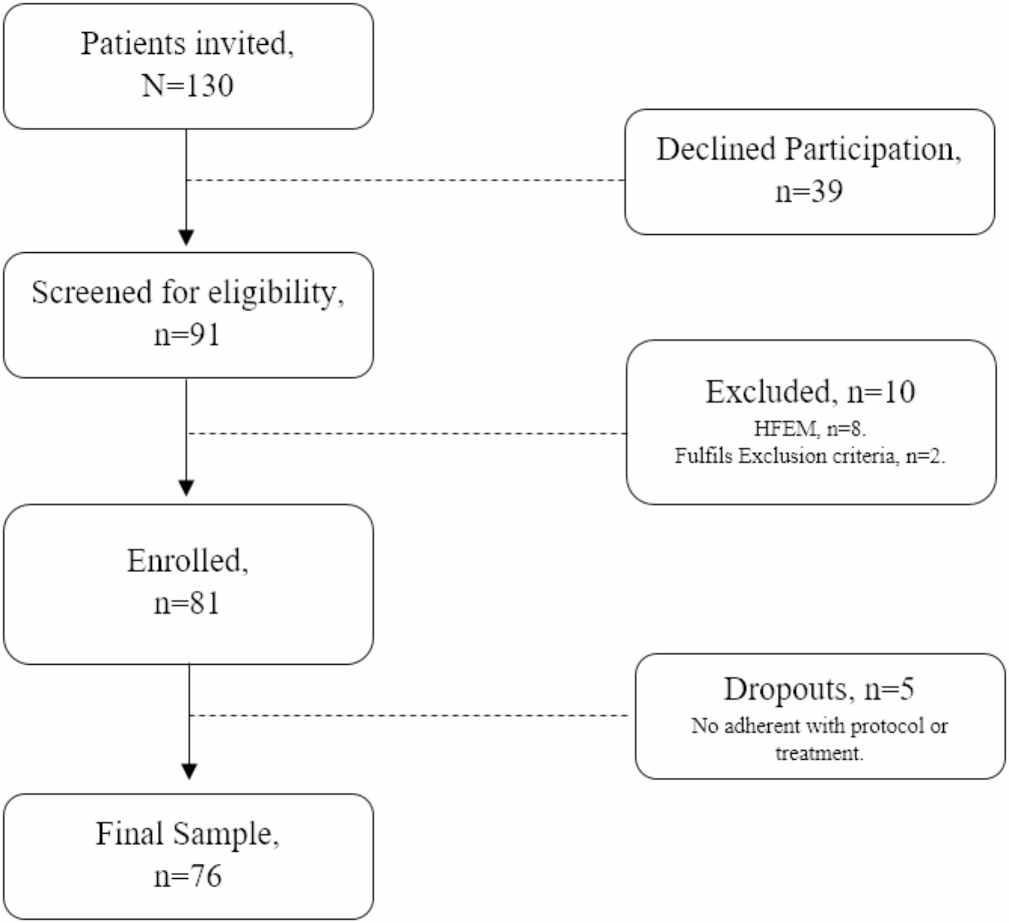
Participants

The flowchart of the recruitment and participant selection/exclusion is presented in Fig. 1.

Fig. 1

Flow chart of the study showing the number of participants approached, included, and completing valid sessions. Invalid sessions were those scheduled as preictal but not followed by an attack within 72 hours, as well as sessions from participants excluded after an incidental finding was detected during the MRI exam

The recruitment of patients with migraine was performed by a neurologist during routine medical consultations at the headache outpatient clinics of Hospital da Luz. We did not perform a statistical power analysis before initiating the study. Nevertheless, we targeted a sample size of 15 migraine patients, consistent with prior MRI cohort studies that identified group differences during spontaneous migraine attacks with sample sizes of N = 13 (Coppola et al., 2016, 2018) or N = 17 (Amin et al., 2018). Healthy control participants, comprising adult females, were recruited through social media advertisements targeting the general population and university campus, ensuring they matched the clinical sample in gender, age, contraceptive use, and menstrual phase at the time of scanning. The inclusion criteria for the participants were the following: having an age between 18 and 55 years; having at least 9 years of education; Portuguese being their first language; being healthy (excluding migraine, for the patients), without any diagnosed condition significantly hindering active and productive life or causing life expectancy to be below 5 years; suffering from low-frequency episodic migraine without aura, diagnosed according to the criteria of the 3rd edition of the International Classification of Headache Disorders (ICHD-3) (International Headache Society, 2018) with menstrual-related migraine attacks (for patients only). The exclusion criteria were: history or presence of a neurologic condition (excluding migraine, for the patients); history or presence of a psychiatric disorder and/or severe anxiety and/or depressive symptoms as indicated by questionnaires; history or presence of vascular disease; receiving treatment with psychoactive drugs, including anxiolytics, antidepressants, anti-epileptics, and any migraine prophylactics; being pregnant or trying to get pregnant, breastfeeding, being post-menopausal, or using contraception precluding cyclic menses; contraindications for MRI. An initial pool of 29 migraine patients and 60 controls were approached out of which 18 and 16 were included in the study, respectively.

We aimed to study the migraine cycle (between peri-ictal and interictal phases) longitudinally, in a specific stage of evolution of the disease in each patient. Data was acquired from 18 female patients that we planned to assess in 4 sessions: preictal (M-pre), ictal (M-ict) and postictal (M-post) phases (around menses), and interictal phase (M-inter) (post-ovulation). The preictal session was acquired within a window of 72 hours preceding the onset of a spontaneous migraine attack (Giffin et al., 2003; Stankewitz A et al., 2011). For each patient, we scheduled the preictal session based on the usual migraine attack onset in relation to menstruation and their prediction of menses start. A preictal session was considered valid upon confirmation with the patient after 72 hours that a spontaneous migraine attack had occurred during the period following our assessment. Considering this, 3 sessions were deemed invalid and discarded because during the 72 hours follow-up to confirm the occurrence of a spontaneous migraine attack it was found that the attack had not taken place. The postictal session was acquired within 48 hours after pain relief from the spontaneous migraine attack (International Headache Society, 2018). Given that some patients struggle to recognize their symptoms (Gago-Veiga et al., 2018; Schulte et al., 2015) and functional changes may occur even before symptoms become apparent, we relied solely on the temporal criteria, which were consistently applied across all patients. For the interictal session, participants had to be free from pain for at least 48 hours before, with confirmation of the absence of a migraine attack obtained 72 hours post-scan. Of the 18 patients, one was excluded due to an incidental finding. Only 10 migraine patients (M group) completed the 4 sessions and were included in the analysis. The demographic and clinical data are presented in Table 1. The attack features concern a typical migraine attack, not being specific to the examined ictal session.

Furthermore, we collected data from 16 healthy controls matched for gender, age, contraceptive use, and menstrual phase at the time of scanning. One subject was excluded due to an incidental finding and another one due to technical issues during the recording. Therefore, the final sample included 14 healthy controls (HC group). They were assessed in two phases of the menstrual cycle to match the peri-ictal and interictal phases of the patients, yielding respectively the perimenstrual phase (HC-pm) (approximately 5 days before or after the menses) and the post-ovulation phase (HC-postov) (approximately on day 19 of the menstrual cycle). The demographic data for this group is also presented in Table 1.

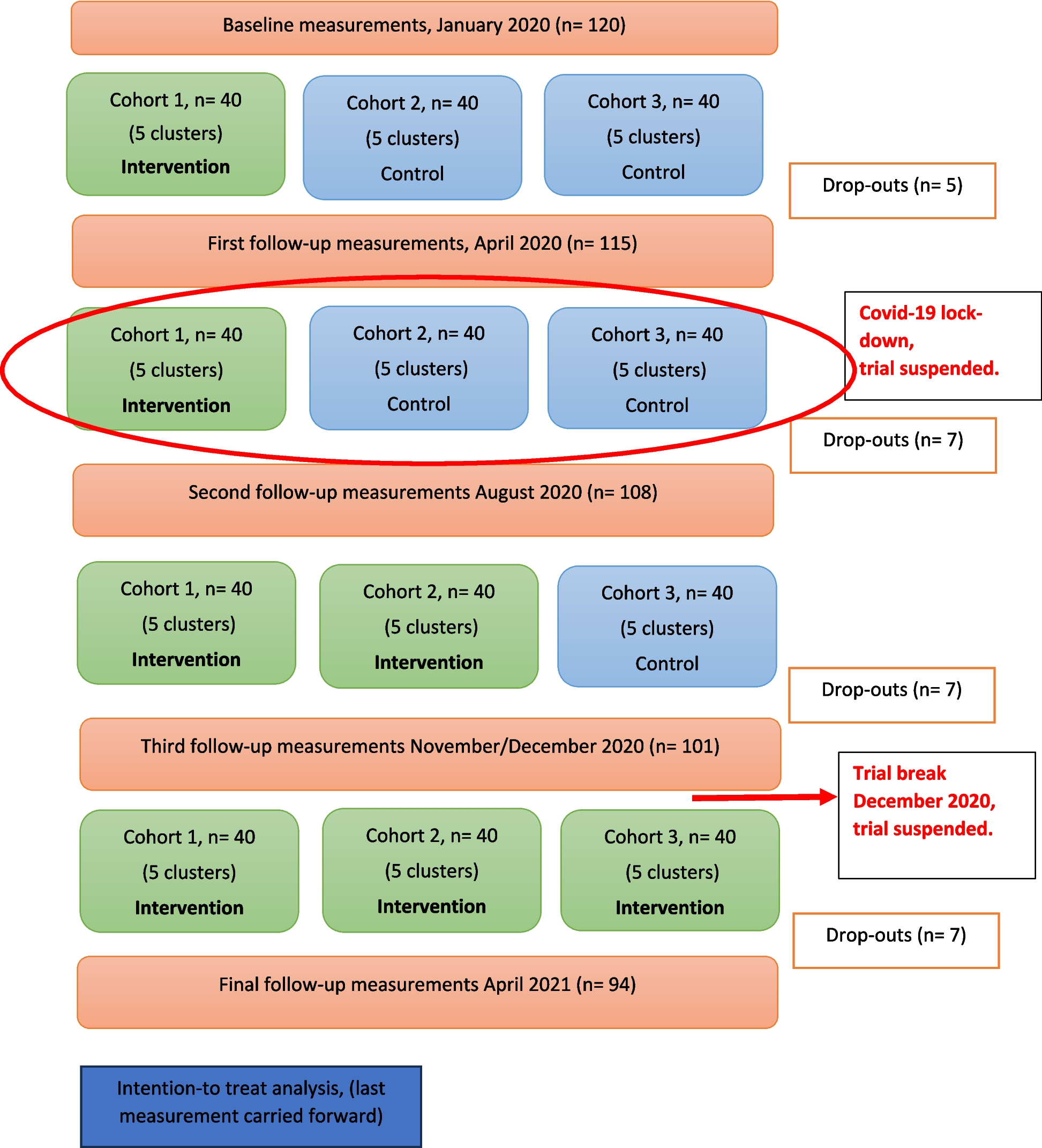
Table 1 Demographic characteristics and migraine clinical features. The median values are presented along with the interquartile range (IQR)

The experimental protocol is schematically represented in Fig. 2. Due to logistic constraints, for each participant the sessions were, in general, performed during different migraine/menstrual cycles. The data acquisition from both patients and controls took place between June 2019 and December 2022. All scanning sessions were performed in the evening (7:00–9:00 p.m.).

Fig. 2

Definition of preictal (M-pre), ictal (M-ict), postictal (M-post) and interictal (M-inter) phases for the migraine patients (M) and the corresponding phases for the healthy controls (HC), matched for the menstrual cycle, perimenstrual (HC-pm) and post-ovulation (HC-postov). The symptoms illustrated across the migraine cycle are only present for the M group and include sleepiness, food cravings, increased sensitivity to light/sound, mood changes, cognitive dysfunction, fatigue, and thirst

MRI data acquisition

The MRI data was acquired using a 3T Siemens Vida system, using a 64-channel radio frequency (RF) coil. Functional images were obtained using a T2*-weighted gradient-echo Echo Planar Imaging (EPI) with the following parameters: repetition time (TR)/echo time (TE) = 1260/30ms, flip angle = 70º, 60 slices, 2.2 mm isotropic voxel resolution. We used techniques to speed up the data acquisition, namely, in-plane generalized autocalibrating partially parallel acquisition (GRAPPA) acceleration factor = 2 and simultaneous multi-slice (SMS) factor = 3. High resolution structural images were acquired with a T1-weighted magnetization-prepared rapid gradient echo (MPRAGE) sequence, with TR = 2300 ms, TE = 2.98 ms, inversion time (TI) = 900 ms, and 1 mm isotropic voxel resolution. To improve image quality, we also captured fieldmap magnitude and phase images using a double-echo gradient-echo sequence (TR = 400.0 ms, TE = 4.92/7.38 ms, voxel size: 3.4 × 3.4 × 3.0 mm3, flip angle = 60º), which helps correct for distortions caused by magnetic field variations. Participants were instructed to keep their eyes open, looking at a black screen, and to not think about anything in particular for 7 min (333 fMRI volumes). To mitigate acoustic noise exposure and minimize head motion, earplugs were used and small cushions were placed beneath and on the sides of the head of the subject.

MRI data preprocessing

The MRI data was preprocessed using FMRIB Software Library (FSL)’s tools (Jenkinson et al., 2012).

Structural images were preprocessed to remove non-brain tissue using Brain Extraction Tool (BET) and corrected for bias field inhomogeneities using FMRIB's Automated Segmentation Tool (FAST). Each structural image was then aligned to the subject's functional space (reference volume) as well as the standard Montreal Neurosciences Institute (MNI) space using FMRIB's Linear Image Registration Tool (FLIRT) and FMRIB's Non-Linear Image Registration Tool (FNIRT). White matter (WM) and cerebrospinal fluid (CSF) masks were derived by tissue segmentation using FAST (a threshold equal to 1 was applied to the obtained tissue probability maps), and subsequently registered to the functional space. The CSF mask was further refined by intersecting it with the lateral ventricles (originally in the MNI space and transformed to the subject’s functional space) was performed.

fMRI preprocessing consisted of: distortion correction based on the acquired fieldmap; volume realignment; high-pass temporal filtering with a cut-off frequency of 0.01 Hz to remove slow drift fluctuations; regression of motion parameters, WM, CSF and motion outliers in a single step; spatial smoothing was employing a Gaussian kernel with a full-width half maximum of 3.3 mm. The code used for fMRI preprocessing is available here: https://github.com/martaxavier/fMRI-Preprocessing.

MRI data analysis

The framework used for data analysis is inspired by the work of Amico & Goñi (2018), in which principal component analysis (PCA) is applied in the connectivity domain and the individual FC are then reconstructed using the number of principal components (PCs) that maximizes identifiability, i.e. how similar a subject is to himself/herself and how different he/she is from other subjects. We extend this to a novel multilevel clinical connectome fingerprinting framework in which identifiability is maximized over three levels: within-subject, within-session and within-group. Therefore, in this study, the concept of identifiability is expanded to encompass the ability to distinguish unique FC patterns at various levels, including individual subjects, specific sessions, or distinct groups. This approach offers a novel perspective on brain connectivity by focusing on level-specific patterns of functional networks and their distinguishability, rather than solely examining shared or common patterns as usually done in FC analysis. The resulting FC fingerprints are then used for two separate analyses: computing the correlation among them within-subject, within-session and between-group, and performing Network-Based Statistic (NBS) analysis for within/between-group comparisons. By adding network-based FC analysis, we can uncover alterations in specific parts of the connectome and more directly relate our findings with previous FC studies, offering a complementary perspective to the FC fingerprinting analysis. Finally, the association between the results of both analyses and clinical features for the M group were investigated. The schematic pipeline representing the workflow employed to perform these steps is depicted in Fig. 3. The code was implemented in MATLAB software version R2016b and is available in https://github.com/isesteves/multilevel-fingerprinting_migraine.

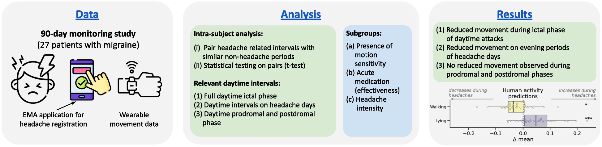
Fig. 3

Pipeline scheme: A. Parcellation into cortical regions of intrinsic networks, based on the Schaefer atlas (100 regions, representing 7 networks) and subcortical and cerebellar regions from the AAL116 atlas: fronto-parietal (FPN), default mode (DMN), dorsal attention (DAN), limbic (LN), ventral attention (VAN), somatomotor (SMN), visual (VN), subcortical (SUB) and cerebellar (CRB). The parcellated data is used for FC computation, by calculating the Pearson correlation between the average time-courses of each pair of regions; B. The lower triangular matrix (excluding the diagonal) of each FC matrix was vectorized and they were all concatenated for PCA decomposition and reconstruction varying the number of PCs N, for each sample k, using the corresponding weights w and mean μ; C. Multilevel clinical connectome fingerprinting framework with PCs selection using a multilevel identifiability matrix corresponding to the Pearson correlation between vectorized FC matrices for all possible combinations of subjects/sessions (samples). In this matrix, for each level, Iwithin corresponds to the average of the elements in dark gray, Iothers corresponds to the average of the elements in light gray and Idiff (%) corresponds to 100×(Iwithin-Iothers). The FC fingerprints are obtained by reconstructing the data using only the selected number of PCs; D. FC fingerprint correlation was computed within-subject, within-session and between-group by averaging the correlation values per subject for each of these cases; E. Computation of Network-Based Statistic (NBS) for within- and between-group FC analysis. F. Association of identifiability metrics and average FC significant edges (found with NBS) with clinical features, using Spearman correlation.

Functional connectomes (FC)

fMRI data was parcellated by computing region average time courses using Schaefer atlas (Schaefer et al., 2018) with 100 parcels, directly corresponding to the 7 intrinsic networks defined by Yeo et al. (2011): fronto-parietal network (FPN), default mode network (DMN), dorsal attention network (DAN), limbic network (LN), ventral attention network (VAN), somatomotor network (SMN) and visual network (VN). Furthermore, given the importance of subcortical regions for migraine, as well as the cerebellum, two additional networks were retrieved from the Automated Anatomical Labelling 116 (AAL116) atlas (Tzourio-Mazoyer et al., 2002): one comprising the hippocampus, amygdala, caudate, putamen, pallidum and thalamus (SUB) and another one comprising 9 bilateral cerebellar regions and the vermis (CRB). Care was taken to ensure that regions overlapping less than 50% with the fMRI data coverage were excluded from further analysis. This procedure led to the bilateral exclusion of 4 cerebellar regions: Crus II, Cerebellum7b, Cerebellum8 and Cerebellum9, for all subjects. Overall, the 9 networks encompassed a total of 130 regions (Fig. 3.A). The time series of each region were demeaned and bandpass-filtered from 0.01 to 0.1 Hz using a 2nd order Butterworth filter. Symmetric FC matrices (130 regions×130 regions, 16900 edges) were generated by computing the Pearson correlation coefficient for each pair of regions.

Principal Component Analysis (PCA)

For each subject and session, the lower triangular part of the FC matrix (excluding the diagonal) was vectorized (8385 edges x 1). The individual FC vectors (10 M subjects × 4 M sessions = 40 samples; 14 HC subjects × 2 HC sessions = 28 samples; total = 68 samples) were concatenated across all subjects and sessions into a single FC matrix (8385 edges×68 samples) (Fig. 3.B). Subsequently, PCA was applied to obtain a number of PCs equal to the number of samples (i.e., 68 PCs), which were ordered by decreasing explained variance. We expect that higher variance PCs will contain global FC information (session- and group-level), intermediate variance PCs will contain subject-level information, and the lowest variance PCs will capture confounding effects, noise and artifacts. Consequently, the FC matrix was reconstructed by using an increasingly larger number of PCs (starting with the largest explained variance), from 2 to 68 for our multilevel clinical connectome fingerprinting approach.

Multilevel clinical connectome fingerprinting framework Multilevel identifiability matrix

Previous fingerprinting studies assessed subjects in at most two sessions (test and retest), either by evaluating them on two different days or by splitting single-day data into two halves. In contrast, the present study assesses the M group in 4 time points and the HC group in 2 time points. To account for the larger number of sessions, we built a modified identifiability matrix by computing the Pearson correlation between all possible pairs of subjects/sessions (see Fig. 3.C). This multilevel identifiability matrix is organized by subject: the first 40 rows/columns correspond to M, with each group of 4 being M-pre, M-ict, M-post and M-inter for each of the 10 M; the last 28 rows/columns correspond to HC, with each group of 2 being HC-pm and HC-postov for each of the 14 HC (68 samples x 68 samples). Hence, unlike the originally proposed identifiability matrix, this modified version is symmetric. For ease of interpretation and to differentiate it from the original, we display our multilevel identifiability matrix by using only the corresponding lower triangular matrix.

Multilevel differential identifiability

The FC fingerprinting framework is based on the premise (already substantiated by evidence) that a subject’s FC profile is more similar to their own FC profile assessed on a different day or task than to those of other subjects (Finn et al., 2015, 2017). The original framework introduced self-identifiability (Iself) as the Pearson correlation between two sessions of the same subject (Amico & Goñi, 2018). Besides within-subject similarity, we extend this differential identifiability concept to consider within-session and within-group similarity. To accommodate the different levels of similarity, we propose the use of within-identifiability (Iwithin), a broader concept which corresponds to the average Pearson correlation between FC matrices belonging to the same subject, the same session, or the same group. Correspondingly, for each of the levels, the elements that are not included in Iwithin are considered Iothers, i.e., average Pearson correlation between different subjects, different sessions, or different groups. The differential identifiability for each level is defined as the difference between these two terms: Idiff (%) = 100×(Iwithin-Iothers) (Fig. 3.C). The higher the Idiff, the more pronounced the fingerprint along that specific level. In this case, instead of maximizing only the within-subject Idiff, we aim for a balance that simultaneously achieves higher values for within-subject, within-session and within-group Idiff. In other words, we manually selected the number of PCs used for the PCA reconstruction that provided the best trade-off across all Idiff levels. Having selected the number of PCs, we consider that the final reconstructed individual FC matrices correspond to the individual FC fingerprints.

FC fingerprint correlation

Upon obtaining the individual FC fingerprints, our goal was to interpret the results in the context of the longitudinal assessment of the M group relative to HC. We extracted Pearson correlation values from the multilevel identifiability matrix computed on individual FC fingerprints, in order to average them for different comparisons and examine their distribution (see Fig. 3.D). These individual FC fingerprints correspond to the matrices of Pearson correlation coefficients between all pairs of brain regions (i.e., involving all connections within and between all networks), after the reconstruction with 19 PCs only. First, within-subject, by separately analysing M subjects (averaging 6 values for each subject, corresponding to combinations of 4 sessions, two by two) and HC subjects. Second, within-session, considering all the points that correspond to either M-pre, M-ict, M-post or M-inter for the M group, and HC-pm and HC-postov for the HC group. For each subject and session, we extracted the correlation values with the rest of the subjects in the same session and averaged them. Third, between-group, considering all the correlation values between each M session and the corresponding HC session: M-pre vs HC-pm, M-ict vs HC-pm, M-post vs HC-pm and M-inter vs HC-postov. For each subject in the M group and session, we extracted and averaged the correlation values with all the other subjects in the corresponding session of the HC group.

Due to the limited sample size, non-parametric statistical tests were used. Specifically, for comparisons within the M or HC group, we applied the signed rank Wilcoxon test. For comparisons between the M and HC groups, conducted specifically for matching sessions (M-pre, M-ict, M-post compared to HC-pm; M-inter compared to HC-postov), we employed the Wilcoxon rank sum test. The significance level was set to α = 0.05 and multiple comparisons were corrected for the false-discovery rate (FDR) with the Benjamini-Hochberg method (Benjamini & Hochberg, 1995) using the Multiple Testing toolbox (Martínez-Cagigal, 2021). For the analysis of FC fingerprints average correlation within-session we corrected for the performance of 11 tests, and for the between-group analysis we corrected for 6 tests.

FC Network-Based Statistic (NBS) analysis

Using the previously obtained individual FC fingerprints for each subject and session, we employed NBS to test for differences in the FC strength (Fig. 3.E). This is a cluster-level tool for human connectome statistical analysis that models FC as a graph and controls for family-wise error rate (FWER) when performing mass univariate testing, which is available as a MATLAB toolbox (Zalesky et al., 2010). The NBS analysis detects network components that consist of connections surpassing a certain threshold. Subsequently, permutation testing is carried out to establish a p-value adjusted for FWER for each network, considering its size. The advantage of performing NBS lies in its ability to identify statistically significant patterns of connectivity across entire networks, rather than isolated connections, providing a more robust statistical approach than performing multiple univariate analysis. The initial threshold for the test statistic was established at a t-value of 4.0, and 5,000 permutations were executed to identify a network component with a p-value < 0.05 after correction for FWER.

Association with clinical features

We investigated the association of FC identifiability and FC strength with relevant clinical features (Migraine Onset, Disease Duration, Attack Frequency, Attack Duration and Attack Pain Intensity), using Spearman correlation (Fig. 3.F), with a significance level of α = 0.05 and multiple comparisons FDR correction with the Benjamini-Hochberg method (Benjamini & Hochberg, 1995; Martínez-Cagigal, 2021).

Regarding identifiability, we evaluated the association with: 1) within-subject average correlation, 2) between-group average correlation for each M session of each patient; 3) between-group average correlation computed across all sessions for each patient. For FC strength, we tested the association with the average FC across all edges that showed significant differences when comparing M and HC, for each patient. In the association with clinical variables, for each case we corrected for the number of clinical variables (5 tests). Additionally, for point 2) we also corrected for the number of sessions (4 tests).