Most participants completed the task on their personal computers (PCs), and the remainder completed the task on their tablets (PC, 62 participants; tablets, 13 participants) (Supplementary material 1: Table S1). The participants accessed Pavlovia (pavlovia.org) to complete the experimental task, which was developed using PsychoPy v2021.2.3. The stimuli used in the task (aliens, treasures, and backgrounds) were adapted from open-access materials created by Kool et al. [30], whereas the other stimuli (rockets) were adapted from an online site (iStockphoto.com).

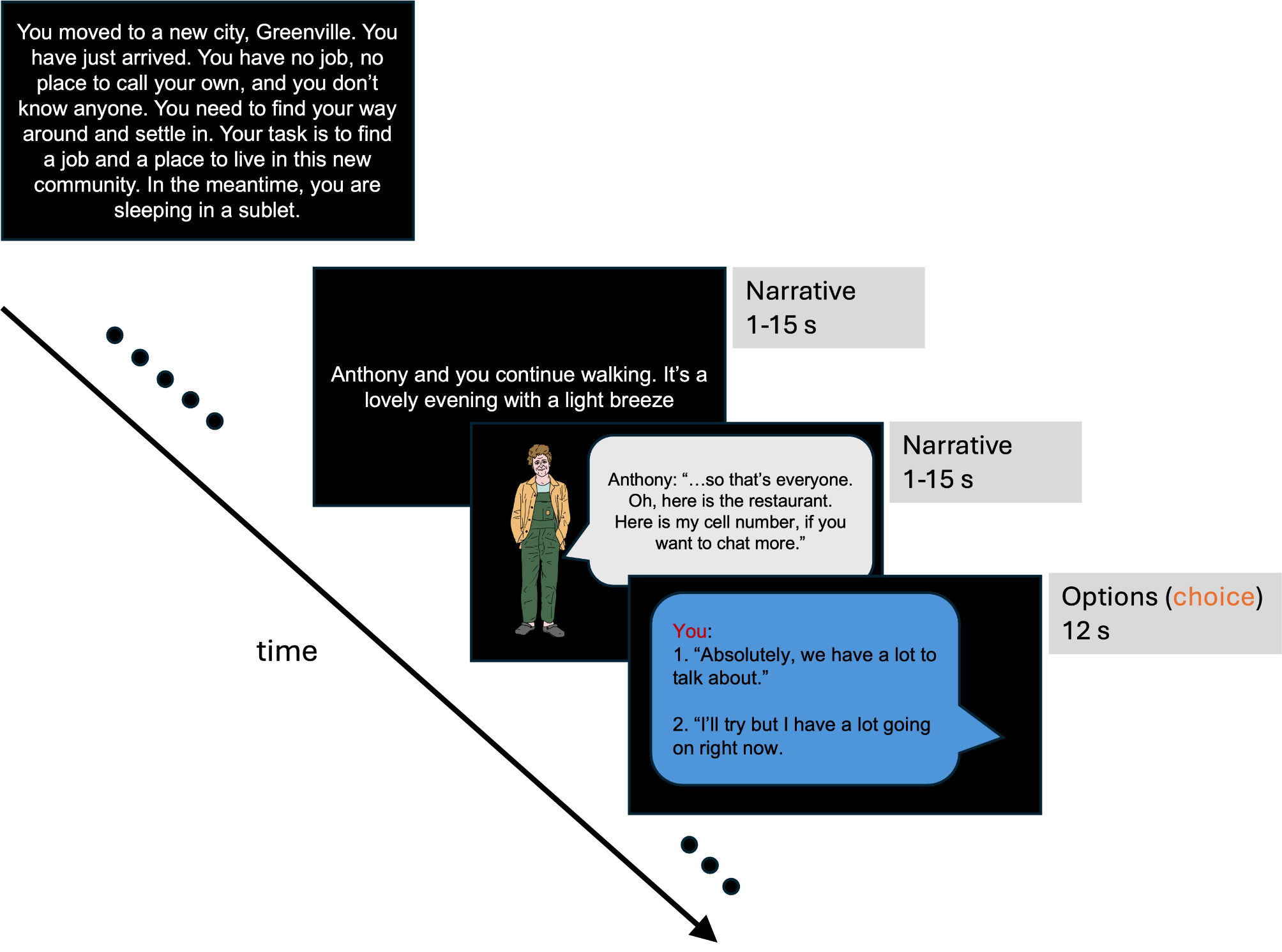
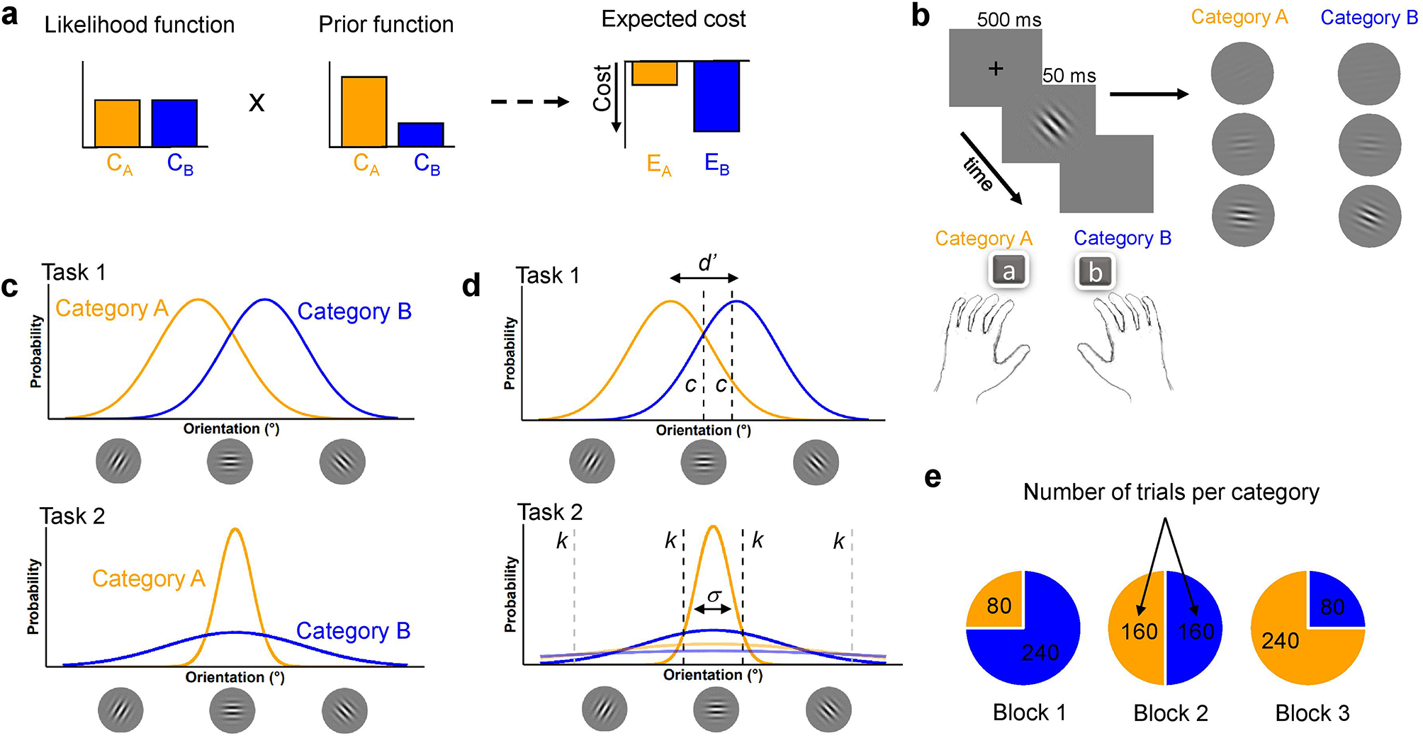
Experimental task

In this study, we created a treasure task based on the risk-sensitive reinforcement learning task of Rosenbaum et al. [17] (Fig. 1). As a cover story, the participants rode a rocket to a planet and received treasures from an alien who gave them 0–8 treasures. The number of treasures the participants received depended on the rocket they chose, and their challenge was to collect as many treasures as possible and obtain the large rocket. There were five rockets, including three deterministic rockets for 0, 2, and 4 treasures, respectively, and two probabilistic rockets for 0 or 4 and 0 or 8 treasures, respectively (50% each). In the task, there were 3 blocks and 183 trials, including 42 sure vs. risky choices (24 choices for a 100% 2-treasure rocket vs. a 50% 0- or 4-treasure rocket and 18 choices for a 100% 4-treasure rocket vs. a 50% 0- or 8-treasure rocket), 24 other choices (a 100% 2-treasure rocket vs. a 50% 0- or 8-treasure rocket), 42 test choices that ensured that participants learned the features of each rocket (e.g., a 100% 2-treasure rocket vs. a 100% 4-treasure rocket), and 75 forced-choice trials in which participants were forced to learn the features of each rocket. The trial order was pseudo-randomized based on seven templates created from the order of the seven participants in the study by Rosenbaum et al. [17].

Fig. 1Basic analysisRisk preference

First, we compared group differences in risk preference using a t-test. Subsequently, using multiple regression analysis, we examined whether there was a group difference in risk preference that changed nonlinearly with age by modeling the interaction term of the quadratic term of age and groups. As confounding covariates, in addition to the reported gender (male, female, or preferred not to report) and execution device (PC or tablet), we modeled the accuracy of the test trials in the second and third blocks, which was significantly correlated with IQ scores among participants who reported their IQ score (r = 0.34, p = 0.012), to remove the effect of the intellectual component associated with this task. Accordingly, the interaction term of the quadratic term of age and groups, interaction term of age and groups, execution device, reported gender, and accuracy of the test trials were modeled. Models were assessed using the lm_robust command from the "estimatr" package [31] with heteroskedasticity-consistent 0 robust standard errors. This method estimates the standard errors under heterogeneous variances and allows for valid inference even when the assumption of constant variance is violated. In these analyses, categorical variables were coded as 1 = AUT and − 1 = NTP for the group and as 1 = PC and − 1 = tablet for the device; continuous variables (age and accuracy) were scaled to mitigate multicollinearity issues. We checked for the multicollinearity of regressors within models using the “performance” package [32], and confirmed that the variance inflation factor (VIF) of each regressor did not exceed 10, while VIF values greater than 10 are a sign of high, unacceptable correlation of model predictors.

Furthermore, as a consecutive analysis to confirm the nonlinear developmental change in risk preference in each group, we conducted a multiple regression analysis for risk preference within each group using the model with the quadratic term of age, in addition to linear term of age, reported sex, execution device, accuracy of the test trials, and SCQ score.

Stay probability

We calculated the stay probability (i.e., the probability of choosing the same option consecutively) of the sure and risky choices both after the rewarding and non-rewarding outcomes. In these calculations, we did not consider the outcome of the forced-choice trials that appeared between the re-risk choice trials. We investigated the group differences in each stay probability that changed nonlinearly with age by modeling the interaction term of the quadratic term of age and groups. The other regressors were the same as those used in the analysis for risk preference. Furthermore, as a consecutive analysis to confirm the nonlinear developmental change in each stay probability in each group, we conducted a multiple regression analysis within each group using the same regressors as in the analysis for risk preference.

Computational modelingModel description

In this study, we fit three widely used models, the Q-learning (QL), utility, and risk-sensitive QL (RSQL) models [16,17,18], and our proposed model, the surprise model [18]. For each model, the learning rate was constrained to the range, 0 ≤ α, α+, α− ≤ 1, with a beta (2,2) prior distribution, and the inverse temperature was constrained to the range, 0 ≤ β ≤ 20, with a gamma (2,3) prior distribution. The utility parameter was constrained to the range, 0 ≤ ρ ≤ 2.5, with a gamma (1.5,1.5) prior distribution. Additionally, the modulation rate of the surprise model was constrained to − 1 ≤ d ≤ 1 with a uniform prior distribution.

QL model

The QL model was used as the base model for the other three models. The QL model incorporates the Rescorla-Wagner rule, where only the Q-value of the chosen option is updated based on a prediction error that explains the observed behavior by computing the action value Q(t) for each trial t, which represents the expected outcome of the action. The Q-value of the chosen action is iteratively updated based on a prediction error, which is the difference between the expected outcome Q(t) and the received outcome r, by a learning rate α.

$$Q\left(t+1\right)=Q\left(t\right)+ \alpha \left(r\left(t\right)- Q\left(t\right)\right)$$

Utility model

The utility model is a QL model that incorporates nonlinear subjective utilities for different amounts of rewards. In this model, the reward outcome is exponentially transformed by ρ, which represents the curvature of the subjective utility function for each individual.

$$Q(t+1)=Q(t)+ \alpha (^- Q(t))$$

RSQL model

In the RSQL model, which is a QL model, positive and negative prediction errors have asymmetric effects on learning. Specifically, there are separate learning rates: α+ and α− for positive and negative prediction errors, respectively.

\(Q(t+1)=Q(t)+ ^(r(t)- Q(t))\) for positive prediction error

\(Q(t+1)=Q(t)+ ^(r(t)- Q(t))\) for negative prediction error

Surprise model

In the surprise model, the received outcome r is affected by surprise (absolute value of the prediction error). In this model, S(t) is the subjective utility modulated by surprise. The degree of modulation is controlled by the parameter d as follows:

$$S\left(t\right)=r\left(t\right)- d\left|r\left(t\right)- Q\left(t\right)\right|,$$

$$Q\left(t+1\right)=Q\left(t\right)+ \alpha \left(S\left(t\right)- Q\left(t\right)\right).$$

For all models, the probability of choosing option i during trial t is provided by the softmax function:

$$P\left( \right) = \frac}\left( \left( t \right)} \right)}}}^ }\left( \left( t \right)} \right)}} ,$$

where β is the inverse temperature parameter that determines the sensitivity of the choice probabilities to differences in the values, and K represents the number of possible actions (in the present study, K = 2); moreover, a(t) denotes the option chosen in trial t.

Parameter estimation

We fit the parameters of each model using the maximum a posteriori (MAP) estimation, which improves parameter estimates by incorporating prior information on parameter values [33, 34]. We also approximated the log marginal likelihood (model evidence) for each model using the Laplace approximation [35]. We used the R function “solnp” in the “Rsolnp” package [36] to estimate the fitting parameters.

Model comparison

For model selection, the model evidence (log marginal likelihood) for each model and participant was subjected to random-effects Bayesian model selection (BMS) using the "spm_BMS" function in SPM12 [37]. BMS provides a less biased and statistically more accurate way to identify the best model at the group level by estimating the protected excess probability, which is defined as the probability of a particular model being more frequent in the population among a set of candidate models [34]. We conducted a model comparison for all participants in each group. To visualize how well the winning model fit the data, we also determined the number of participants that best fit each model [34].

Estimated parameters

After the model comparison, we investigated group differences in the estimated parameters of the winning model, which changed nonlinearly with age, by modeling the interaction term of the quadratic term of age and groups. The other regressors were the same as those used in the risk preference analysis. Furthermore, as a consecutive analysis to confirm the nonlinear developmental change in the estimated parameters in each group, we conducted a multiple regression analysis within each group with the same regressors as in the risk preference analysis.

Parameter and model recovery

We conducted parameter recovery to assess the reliability of parameter estimation procedures; specifically, we determined how accurately parameters were estimated when the true generative model and its parameter values were known [34, 38, 39]. Model recovery was performed to test the discriminability of each model [34, 38, 39]. Details of each analysis are provided in Supplementary material 1 (Supplementary material 1: Text S1, S2).

Posterior predictive check

We performed a posterior predictive check that analyzed the simulated data in the same way as the analyses of the empirical data to validate that each model adequately captured behavioral data [34, 40].Detailed information of the analysis is provided in Supplementary material 1 (Supplementary material 1 Text S3).

Supplemental analysis with open data

As the task used in this study was based on the study by Rosenbaum et al. [17], to confirm that the surprise model was better fitted to the risk preference data with similar age diversity, we conducted model fitting and model comparisons. For model fitting, the parameters were set to be the same as those used in this study. Additionally, to confirm the nonlinear relationship between age and the surprise parameter, we conducted a regression analysis of the surprise parameter using the quadratic term of the scaled age.