Thirty-four adults diagnosed with autism (28 males and 6 females) and 49 non-autistic individuals (11 males and 38 females) participated in this experiment and received either monetary compensation (40 shekels/hour) or university credit compensation (3 credits/hour). Autistic participants were recruited from a reliable pool of participants routinely completing experiments for the Department of Special Education. The two groups recruited for the experiments matched in age (t(101.66) = 0.548, p = .585), the mean age was m = 26.58 years old, se = 0.90, for the autistic group, and m = 27.21, se = 0.71, for the non-autistic group. The IQ was evaluated using the Test of Non-Verbal Intelligence (TONI-4) measuring cognitive functioning without the interference of language deficits [27]. The two groups matched in IQ (t(60.61) = 0.82, p = .417), with a mean of m = 99.83, se = 11.47 for the autistic group, and m = 101.69, se = 9.91 for the non-autistic group. We used the Autistic Quotient (AQ) questionnaire to evaluate the participants’ autistic traits, and a t-test (t(64.47) = 6.30, p < .001) revealed that the autistic group had a significantly higher AQ, m = 26.89, se = 8.27, compared to the non-autistic group, m = 17.01 se = 6.80. We maintained a minimum 24 h-interval between consecutive experiments for each individual.

The autism diagnosis was confirmed through rigorous criteria, including the DSM-V, the Autism Diagnostic Interview (i.e., ADI-R52), and the Autism Diagnostic Observation Schedule (i.e., ASDOS-2). Moreover, all participants completed the Community Assessment of Psychic Experiences (i.e., CAPE) and AQ questionnaires, in their preferred language (Hebrew or English), either following the experimental phase or before the experiment, during the clinical assessment phase. We excluded non-autistic individuals with a history of epilepsy, neurological, psychiatric, or learning disorders, as well as those currently using psychiatric medications. We excluded individuals diagnosed with autism who have known genetic disorders (e.g., Down syndrome).

Stimuli were programmed in Matlab (The MathWorks, Inc., Natick, MA) with the Psychophysics Toolbox extensions, and were presented on a gamma-corrected 21-in CRT monitor (1280 × 960 resolution, 85-Hz refresh rate). Participants used the keyboard to respond.

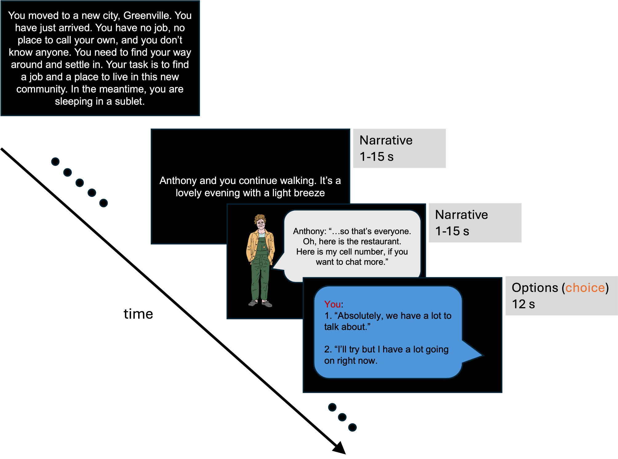
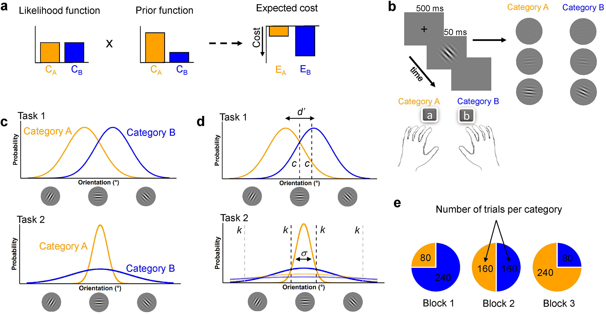
Figure 1b illustrates the stimuli, experimental procedures, and tasks, based on Qamar et al. (2013), Adler and Ma (2018) and Denison et al. (2018). All stimuli were presented against a gray background (50 cd/m2). Each trial began with fixation (a black circle 0.2° of visual angle in diameter) for 500 ms, followed by the stimulus display for a duration of 50 ms. The stimulus was a sinusoidal grating with a two-dimensional Gaussian spatial envelope (i.e., Gabor patch), with sd = 0.325°, 85% contrast, and spatial frequency of 3 cycles per degree, presented at the center of the screen. In each trial, the orientation of the grating was randomly drawn from one of two Gaussian distributions, corresponding to the two stimulus categories (Fig. 1c). Following stimulus offset, participants reported both their category choice (Category A or B) and their level of confidence using a 4-point scale. This confidence rating scale ranged from high-confidence Category A to high-confidence Category B. The confidence data will be the focus of a separate paper. To manipulate the sensory uncertainty, we varied the stimulus contrast, randomly across trials, across seven fixed values (0.004, 0.016, 0.033, 0.093, 0.18, 0.36, 0.72).

Our experimental design incorporated continuous orientation distributions for each choice category, a critical feature enabling the separation of the participant’s sensory noise from their decision rule [26, 28]. Stimulus orientations were drawn from Gaussian distributions with means of mA = 86°and mB = 94° (tilts around vertical), both with standard deviations of sA = sB = 5° (see Fig. 1c, Task 1). The categories were partially overlapping, such that the maximum accuracy level was 80%. Participants were instructed to report which category they thought the stimulus belonged to on every trial, and they did not have any time limit to provide their answers.

To manipulate priors, we varied the base rate of Category B (and conversely, Category A) across three blocks of trials. Two blocks had imbalanced base rates: one with a higher probability for Category A (B = 25% and A = 75%) and the other with a higher probability for Category B (B = 75% and A = 25%). The third block had balanced probabilities (B = 50% and A = 50%). See Supplementary Fig. 1a-c, for a depiction of the frequency of each orientation per category for each base rate block. The neutral block was always performed second. The order of the low and high blocks was counterbalanced between participants. Here, we expected a shift of decision boundary that favored the category with the high base rate (Fig. 1d, Task 1). Participants completed 960 experimental trials over approximately 50 min.

To ensure the comprehension of the main manipulations (i.e., base rate), a “check question” was randomly introduced during the experiment. Participants were asked to hypothetically gamble an amount of money on a category, ranging from 0 to 99 cents, on the chances of the next trial belonging to that category, and that the amount left would be automatically gambled on the other category. They were informed that their predictive performance would determine a monetary/credit bonus in addition to the original compensation.

To ensure that all participants understood the task and manipulations, at the beginning of each experiment we conducted an extensive training phase on the categories and the confidence keys, then on the prior information at the beginning of each block (see Supplementary Methods).

All analyses were performed on R version 4.2.2. Because confidence data was not the focus of the present study, we considered only the categorical response, collapsing across confidence keys.

To validate the manipulation of prior knowledge, we calculated the mean points gambled on category B in each base rate block for each participant. We then conducted a 2 × 3 mixed-design Analysis of Variance (ANOVA) with group (non-autistic, autistic) as the between-subject factor, category B base rate [75% (high for B), 50% (balanced), 25% (low for B)] as the within-subject factor, and points gambled on category B as the dependent variable.

For the main orientation categorization task, we first analyzed the raw data by calculating the probability of reporting category B across 16 binned orientation levels (-14, -12, -10, -8, -6, -4, -2, 0, 2, 4, 6, 8, 10, 12, 14) within each base rate condition. We then conducted a 3 × 16 × 2 mixed-design ANOVA with category B base rate and binned orientations as within-subject factors, and group as the between-subject factor on the probability of reporting B as the dependent variable.

To independently estimate perceptual sensitivity and decision boundary, we utilized the framework of standard signal detection theory (SDT). Sensitivity (d’) reflects the ability to discriminate between the two categories, while the decision criterion (c) indicates the decision bias participants employed to favor one category over the other. We then conducted a 7 × 3 × 2 mixed-design Analysis ANOVA with contrast (0.004, 0.016, 0.033, 0.093, 0.18, 0.36, 0.72) and category B base rate as within-subject factors, and group as the between-subject factor, on both d’ and c.

To assess overall adjustment of decision boundary to a change in category base rate, we computed the shift in c between biased base rate (75% and 25%) blocks Dcriterion = c75% - c25%. We conducted a 7 × 2 mixed-design ANOVA with contrast as within-subject factor and group as between-subject factor, on the Dcriterion.

To account for sensory uncertainty (the inverse of sensitivity) differences across and within subjects when assessing the effect of base rate on the decision boundary, we used an ideal observer analysis approach. We calculated the optimal criterion shift (copt) based on the optimal bias (β), which was calculated for a range of d’ values (Eq. 1). β was derived from the base rate (α) condition (Eq. 2). The parameter α could take a value of α = 0.25 (low base rate) or α = 0.75 (high base rate).

$$\:c_\:}=\frac\text\text\left(\beta\text\:\right)}}$$

(1)

$$\:\beta_}\:=\frac$$

(2)

Participants’ suboptimality cerror was estimated as the difference between a participant’s actual c and the corresponding copt based on their d’ value, for each stimulus contrast. We conducted a 7 × 2 mixed-design ANOVA with contrast and group on the cerror.

In all ANOVAs, significant effects were further investigated using paired and unpaired t-tests as Bonferroni corrections were applied to control for multiple comparisons. The effect sizes were calculated using partial eta square.

In addition, we used a t-test Bayes analysis to assess the evidence for differences between the autistic and non-autistic groups in sensitivity (d’), decision criterion (Dcriterion), and suboptimality (cerror). Bayes factors (BF) were used to quantify the likelihood of the data occurring under assumptions of the alternative hypothesis (H1 = difference between the two groups) over the null hypothesis (H0 = no difference between the two groups). BF < 1 indicates that the data provide evidence in favor of H0. 1 < BF < 3 indicates weak evidence for H1. 3 < BF < 10 indicates moderate evidence for H1. BF > 10 indicates strong evidence for H1 [29].

We also performed linear-mixed effect models to confirm the main effects and interactions of category base rate and contrast on the sensitivity, decision criterion, and deviation from optimality.

Descriptions of analysis on linear mixed effect models, reaction time (RT) data and correlations between AQ and deviation from optimality can be found in Supplementary Methods, and the results are described in Supplementary Results and Supplementary Fig. 2a and 3a-b.

Participants with an accuracy below 0.6 at the three highest contrast levels and across blocks were excluded from all analyses. Participants demonstrating extreme deviation from an optimal observer (cerror > 50) were excluded from the optimality statistical analyses. Participants exhibiting an average reaction time that was three standard deviations away from their group’s mean were excluded from the reaction time analyses (Table 1).