2.1 Dataset

The analyzed data included four seasons (2014/15 to 2017/18) of media-based injury records in the first male German football league, a subset of the dataset used by Aus der Fünten et al. [20]. Injuries were prospectively documented in a standardized manner through an official collaboration with German kicker® sports magazine [21,22,23,24], with team-specific updates provided by assigned journalists. Additionally, injuries were daily monitored through the social media websites of teams and players, as well as the online platform https://ligainsider.de, with occasional reference to http://www.transfermarkt.de. Each injury entry in the database was verified by at least one additional source, and diagnoses were confirmed by medical staff according to international guidelines [14]. Neither research ethics board approval nor a trial registration were required as all data were collected from publicly available sources.

2.2 Equity, Diversity, and Inclusion Statement

The focus of this work is on male professional football. While the specific results are presumably dependent on discipline, performance level, and sex, the method presented may be applied in other settings and populations.

2.3 Data Analysis2.3.1 Pre-processing

A RTP scenario is triggered by an index injury followed by rehabilitation, RTP, and eventually a subsequent injury. As contact and non-contact injuries can equally impact on players’ physical condition and subsequently influence the injury risk after RTP, both categories are considered for the index injury. However, given the unpredictability of physical contact in football, only non-contact time-loss injuries were considered as subsequent injuries. For each player, the first injury on record was considered as the index injury of the following injury, the second injury as the index injury of the third injury. Return-to-play in this study was defined as a full return to training and competition [7].

The severity of index injuries was categorized according to the time loss concept: minimal (1–3 days), mild (4–7 days), moderate (8–28 days), and severe (> 28 days) [14]. The playing position was considered as the players’ main position when the subsequent injury occurred, including goalkeeper, defender, midfielder, and forward. All data processing and following analysis was performed using R Statistical Software (v4.2.2; R Core Team 2022). The knit R Markdown files for data analysis have been made available in the following repository (https://github.com/latilongitude/Injury_risk_after_RTP).

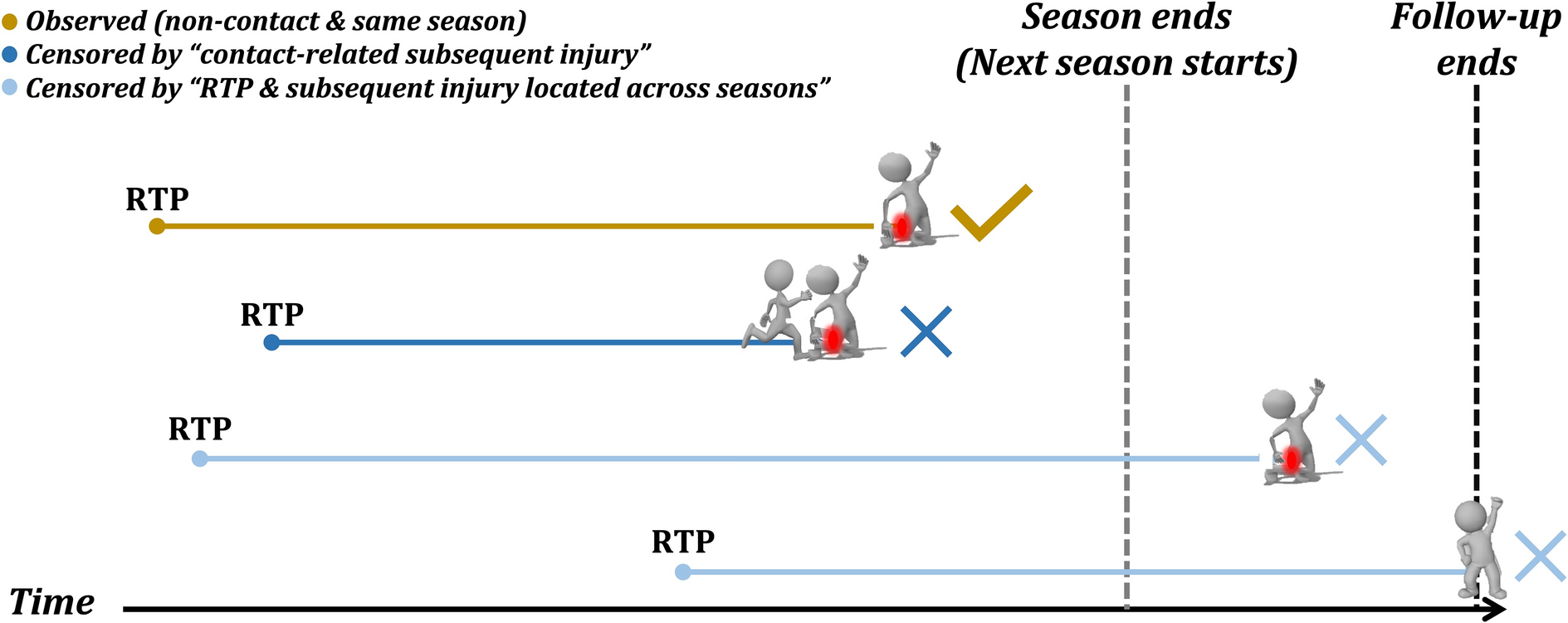
2.3.2 Censoring

Censoring refers to an abbreviated length of follow-up due to the end of the follow-up period or reasons other than the target event. Four football seasons were segmented by the date of the last official match for corresponding season, 23 May for 2014/15 season, 14 May for 2015/16 season, 20 May for 2016/17 season, and 12 May for 2017/18 season. Given that training and match exposure as well as the recording of minor injuries during the summer break might differ from in-season, cases that did not incur a subsequent injury in the same season as RTP were censored at the end of season (date of last match, cp. above and Fig. 1). As this study mainly focused on the occurrence of non-contact injury after RTP, contact-related subsequent injuries equally led to censoring (Fig. 1). A subsequent injury was confirmed as an observed event only when it was observed in both categories (i.e., non-contact subsequent injury occurring in the same season as RTP).

Fig. 1

Two strategies of censoring observations. The example at the bottom is not subsequently injured until the end of the follow-up. RTP return-to-play

2.3.3 Hazard Function

Figure 2 illustrates the steps to derive the continuous hazard function. First, the dataset with censoring information was used to fit a Kaplan–Meier (KM) model [8]. Because of the fine-grained time metric (day), the number of observed events might be trivial for individual time units, which makes the discrete-time KM hazards too volatile to be meaningful. By contrast, at each time \(_\), the cumulative hazard function \(\widehat(_)\) can be derived through an established mathematical relationship (see Eq. 1) from the KM survival function \(}_}(_)\) [13]. The instantaneous risk is the change in cumulative hazard from one time unit (day) to the next, that is, the local slope of the cumulative hazard function. The cumulative hazard function provides a pivot to retrieve continuous hazards as its first derivative [13]. To simplify the calculation, cumulative hazards and time, as response and explanatory variables, respectively, were used to fit a polynomial (tenth degree) regression model. Subsequently, predictions were made for successive days. The rate of change in predicted cumulative hazards was then calculated as the continuous hazard function (i.e., the risk of subsequent injury) [13]. It is important to note that only cumulative hazards from the first 100 days after RTP were used to fit the polynomial.

$$\hat\left( } \right) = - }\hat_}}} \left( } \right).$$

(1)

Fig. 2

Retrieving the hazard function on continuous time. KM Kaplan–Meier

A linear interpolation approach [8] was applied to estimate the median survival time \(T\), as shown in Eq. 2 where \(m\) represents the time interval when the sample survival function is just above 0.5.

$$T = m + \left[ _}}} \left( } \right) - 0.5}}_}}} \left( } \right) - \hat_}}} \left( } \right)}}} \right]\left( \right) - m} \right).$$

(2)

2.3.4 Ancillary Analysis 1: Time Course of Injury Risk Outside of the RTP Context

As detailed in Sect. 1, injury risk is assumed to decline from elevated risks after RTP towards a stable “baseline risk” without systematic dependence on time. While this assumption is highly plausible, it could not be verified directly so far. For comparison, we therefore also applied the above-described method to derive a hazard curve for players not returning from a recent injury. This comparator is based on a time period subsequent to the first 100 days after RTP, which are used to derive the main hazard curve (see Fig. S1-1 in the ESM).

2.3.5 Ancillary Analysis 2: Considering Hierarchical Data Structure

It is important to note that the analyzed dataset features a hierarchical data structure. As players with more frequent injuries (and therefore RTPs) contribute more data points (see Figs. S2-1 and S2-2 of the ESM), these individuals have a disproportionately high impact on the hazard function, leading to potential bias. Aiming to expose the general analytical pipeline for deriving the continuous hazard function as transparently as possible, the nesting of RTP episodes within players is not considered in the above analysis. However, in the ESM, we illustrate and discuss up-sampling and down-sampling, respectively, of the original dataset as two potential options for mitigating this issue while still avoiding advanced modelling techniques.

2.3.6 Ancillary Analysis 3: Round-Robin Splitting to Check Overfitting

To address concerns about overfitting by high-degree polynomial regression, we performed a leave-one-quarter-out data splitting in a round-robin manner. Splitting was performed on the player level and stratified for playing positions to avoid information leakage. The resulting hazard curves were compared with those from the main analysis to probe potential overfitting (see Fig. S3-1 in the ESM).