1 Introduction

Predicting drug combinations is a pivotal task in contemporary medication strategies, focusing on optimizing therapeutic outcomes by anticipating the interactions between different drugs and addressing the limitations of single drugs through predicting interactions between different drugs (Mokhtari et al., 2017). Research on drug combination prediction is of great importance for achieving personalized medicine and enhancing treatment effectiveness (Csermely et al., 2013). With the rapid development of deep learning technologies, the field of drug combination prediction is experiencing significant technological innovations, greatly advancing research in this area (Güvenç Paltun et al., 2021). In 2018, Preuer et al. (2018) developed the DeepSynergy model, marking a significant milestone in the application of deep learning methods for predicting drug combinations. Inspired by DeepSynergy, researchers developed the DeepSignalingSynergy model in 2020 (Zhang et al., 2020), based on a sparse network construction. This model uses neurons in the hidden layer to simulate signaling pathways in cancer cells, assessing each neuron’s contribution to the final prediction through hierarchical relevance propagation (Montavon et al., 2019), thereby enhancing the model’s interpretability. While the DeepSynergy model introduces a novel approach to forecasting drug interactions, it faces limitations when dealing with intricate gene expression profiles and the varied molecular architectures of drugs. Kuru et al. (2021) proposed the MatchMaker model, training a subnetwork for each drug-cell combination. The output latent representations of these subnetworks are concatenated to serve as inputs for another subnetwork, used for predicting synergy scores. Building on this, MARSY (El Khili et al., 2023) also trained two subnetworks representing drug pairs and drug-drug-cell triple combinations; Additionally, CCSynergy (Hosseini and Zhou, 2023) and SynPathy (Tang and Gottlieb, 2022) are drug combination synergy prediction models developed in recent years based on the DeepSynergy model, integrating more types of drug and cell characteristics.

Despite significant progress with deep learning-based drug combination prediction models like DeepSynergy, substantial challenges remain in handling complex gene expression data and drug structural diversity. Subsequent research, such as DrugCell (Kuenzi et al., 2020), has employed more complex network architectures and data processing methods to address these challenges. These methods include advanced dimensionality reduction techniques and modeling for specific biological pathways, aiming to improve the predictive accuracy and biological interpretability. The development and application of Graph Neural Networks (GNNs) (Scarselli et al., 2008) have provided new methods for representing molecular structures and cellular network characterizations. Recent models such as GraphSynergy (Yang et al., 2021), PRODeepSyn (Wang et al., 2022), MOOMIN (Rozemberczki et al., 2022), and KGE-DC (Zhang and Tu, 2022) apply GNNs to drug combination synergy prediction, offering new methods to better capture the intricate interactions and relationships within the data.

While deep learning approaches have achieved some progress in predicting drug combination synergy, they exhibit limitations, particularly in adequately addressing the spatial distribution characteristics of gene expression data. This oversight leads to an in-complete understanding of the spatial adjacency relationships among genes. Furthermore, the acquisition of structured regularity information concerning drugs, as well as potential associative features between drug molecules, remains insufficient.

To overcome the limitations of current methodologies, we introduce a novel predictive model named DKPE-GraphSYN. The main contributions are as follows:

• DKPE-GraphSYN model: The proposed DKPE-GraphSYN model employs a Dual Kernel Density Estimation (DKDE) and Positional Encoding (PE) Channel Cascade Algorithm for processing gene expression data. The innovative method encapsulates both locational and weighted probability density information, thereby effectively capturing the spatial distribution and weights of genes within cellular responses.

• Graph Representation of Drug Molecules: By representing drug molecules using a graph structure, our model captures the potential associations between drug molecules, enhancing our understanding of their interactions.

• Integration of Convolutional Neural Networks (CNN) and GNN: The DKPE-GraphSYN model integrates CNN with GNN to effectively capture associative features between cell lines and drugs, thus enhancing the accuracy of predicting drug combination effects.

2 Materials and methods

Our research method commenced with dividing the dataset evenly into five parts, proceeding through five phases of training and verification. In each phase, we designated one part as the validation set and used using the rest for training set. This rotation ensures all data serve in validation and training sets. We assess the model’s validation performance in each phase, and the collective findings from all phases culminate in a comprehensive evaluation of the model’s effectiveness.

2.1 Datesets

Gene expression data for human cancer cell lines were obtained from the GDSC (Genomics of Drug Sensitivity in Cancer) database (Yang et al., 2012), a comprehensive repository encompassing cancer genomics and drug sensitivity. We selected data for approximately 1000 cancer cell lines from the GDSC. For each cell line, normalized expression levels of 17,737 genes were recorded, from which we selectively identified 496 landmark genes for our analysis. Additionally, the database converted protein/RNA markers derived from gene expression into numerical sequences, facilitating their analysis through computational methods. Subsequently, these gene expression vectors were normalized to standardize the data range, facilitating further analysis.

Our dataset of drug combinations was gathered from the DrugComb database (Zagidullin et al., 2019) (https://drugcomb.org/), derived from 34 diverse studies including O'NEIL (Merck) (O’Neil et al., 2016), CLOUD and so on. Initially comprising 1,432,351 samples, we selected triples consisting of drug A, drug B, and a cell line. We excluded any samples that lacked complete information on drug names, cell lines, or synergy scores to ensure the dataset contained only complete information for analysis. Additionally, to avoid data redundancy, we identified and removed duplicate triples.

By integrating the GDSC and DrugComb databases at the cellular line level, we have successfully established a balanced benchmark dataset consisting of 25,758 unique drug-drug-cell line combinations.

2.2 Drug synergy reference scores

In this study, we define positive (synergistic) and negative (antagonistic) samples based on four types of synergy scores: Loewe (Loewe, 1953), Bliss (Bliss, 1939), HSA (Me, 1989), and ZIP (Yadav et al., 2015). Synergy scores within the DrugComb database are computed utilizing the SynergyFinder software (Ianevski et al., 2017). Relying on a single type of synergy score for evaluation can introduce inaccuracies. Therefore, we utilize a variety of threshold scores (Loewe, Bliss, HSA, ZIP) for assessment purposes. A sample is only incorporated into the training set when all four scores unanimously classify a drug combination as either a positive or a negative sample. This methodology is designed to provide a more detailed and accurate assessment of drug synergy effects, thereby enhancing the precision and stability of the predictive model.

2.3 Architecture

As shown in Figure 1, DKPE-GraphSYN is composed of the DKDE and PE joint gene expression vector feature extraction module, and a graph structure characterization module for drug molecular structure features. In the dual kernel density gene expression vector module, we introduce a DKDE and PE channel cascade algorithm for the first time (see Algorithm 1 for details). This algorithm captures the weighted density and spatial distribution features of gene expression vector data. By cascading DKDE and PE channels, we generate a DKPE image of the gene expression vector, incorporating both DKDE and PE features, which serves as the input for the CNN.

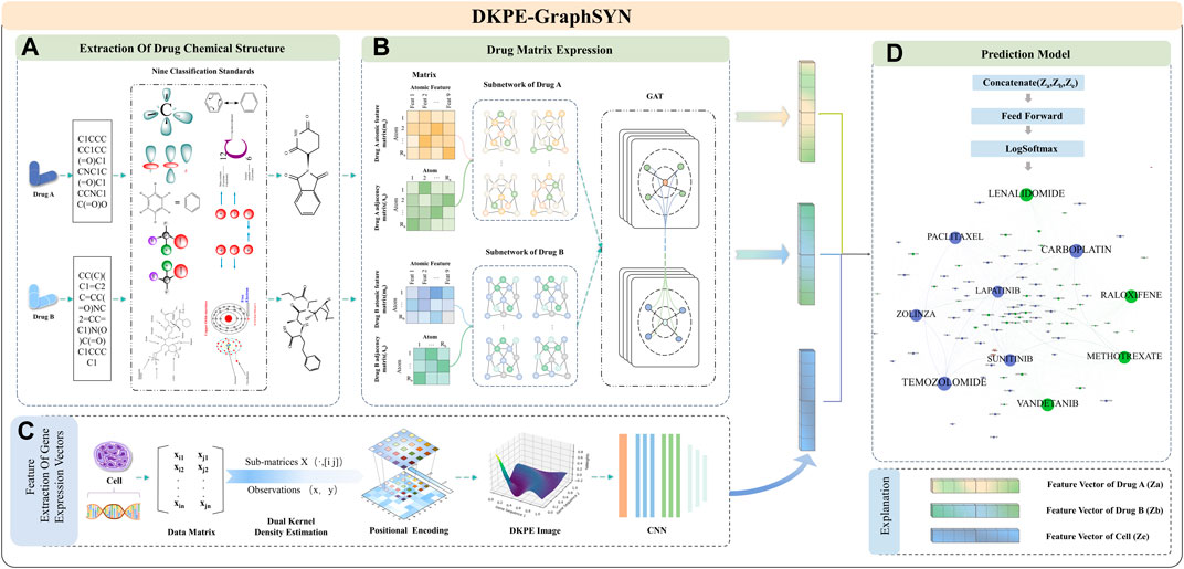
Figure 1. Feature Extraction and Model Training Process of DKPE-GraphSYN. Part (A) The chemical structure of drugs A and B is extracted based on their SMILES representation and nine chemical property classification standards. Part (B) The molecular properties and interactions of the drugs are represented through a graph structure network using matrices. Part (C) Features of the gene expression vector of the cell line are extracted using a DKDE and PE channel cascade algorithm. Part (D) A classification model is constructed by merging the drug and gene expression vector feature vectors, utilizing a feedforward network and the LogSoftmax function to predict the synergistic effects of drugs.

In the graph structure characterization module for drug molecular features, atoms and bonds in the chemical structure of drugs are considered as nodes and edges of the graph (Reiser et al., 2022), respectively. The regularity features of the drug graph structure are then extracted using a GNN. Finally, our model integrates the embedding results from the CNN and GNN, processes them through a feedforward neural network, and outputs the predicted interaction scores between drugs to categorize synergistic and antagonistic interactions.

2.3.1 Feature extraction of gene expression vectors

We propose a DKDE and gene PE for channel cascade integration to comprehensively analyze gene expression vector data, considering not only the weighted probability density of genes but also their spatial distribution. DKDE enhances the understanding of gene pair distributions in gene expression data by integrating calculations from Gaussian kernel functions with estimations of probability distributions, thereby uncovering the weighted probability distribution of gene pairs, and reflecting their interaction strength and spatial distribution characteristics, PE assigns spatial coordinates as numerical codes to each grid point in the DKDE map, to reflect the relative positional relationships and proximal associations of gene expression data in spatial distribution. The channel cascade integration method combines the weighted probability density information of gene expression obtained from DKDE with spatial PE into an enhanced feature matrix. This facilitates convolutional neural networks in concurrently processing and evaluating the spatial distribution characteristics and probability density of genes.

2.3.2 Dual kernel density estimation

In the preprocessing stage of dual kernel probability estimation, representative gene expression vectors are first extracted from the gene expression dataset, with each cell line’s feature vector having a length of 496. Subsequently, each vector is evenly divided into two parts, which are considered as two variables i and j in the data matrix X. A probability distribution matrix is then obtained through the DKDE algorithm. In this matrix, each point represents a weighted probability value of gene expression, indicating a certain probability density, that reflect the interaction strength of specific gene expression pairs. By calculating all points on an equidistant grid, we create a DKDE map, which details the interaction strength of gene expression pairs.

The DKDE algorithm utilizes the Kernel Density Estimation (KDE) function to compute weighted probability densities. This KDE function, a non-parametric statistical approach, is applied to approximate unknown density functions. As illustrated in Figure 2, the algorithm initially extracts columns corresponding to variables i and j from the gene data matrix X, forming an n×2 submatrix X⋅,ij. For every observed value pair x,y within the submatrix X⋅,ij, which denotes gene expression, the value of kernel function K is determined, with the Gaussian kernel selected as K. The formula for calculating the kernel function is shown in Eq. 1:

Ku,v=12π∗⁡exp−0.5*u2+v2,(1)

where u=x−xih,v=y−yjh, with xi and yj being the observed values (i.e., gene samples), and h as the bandwidth. The sum of all kernel function K values is then divided by the product of the total count of observations n and the bandwidth h2, to calculate the value of the bivariate kernel density estimation fij. The calculation process is shown in Eq. 2.

fijx,y=1n∗h2∗∑Kx−xih,y−yjh.(2)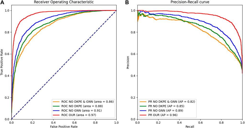

Figure 2. Receiver Operating Characteristic and Precision Recall Curve Comparison. (A) The left panel displays the ROC curves for different model variants, with the AUC metric indicating the ability to distinguish between synergistic and non-synergistic drug combinations. (B) The right panel shows the PR, with the AUPR metric reflecting the precision and recall balance of the models in predicting drug synergies. The ROC and PR curves are essential for evaluating the performance of the ablation study models, demonstrating the impact of the DKPE and GNN components on predictive accuracy.

By repeating the above steps and for all points on an equidistant grid, we obtain the values of the bivariate kernel density estimation fijx,y, which form the DKDE map. This map reveals the interaction strength of gene expression pairs, where fij≠fji indicates the asymmetry of the estimated values, further emphasizing the directional characteristics of interaction strength between gene pairs.

2.3.3 Grid position encoding

Grid Position Encoding forms the core component of our DKDE and PE Channel Cascade Algorithm, designed to precisely capture and describe the complex distribution and interrelations of gene expression data in multidimensional space. By assigning a unique positional encoding to each data point in the DKDE map, we can not only quantitatively analyze the interaction strength of gene pairs but also reveal their spatial relevance in the cellular functional structure.

The procedural steps for applying the PE technique start with identifying the two-dimensional coordinates a,b for each gene expression data point on the DKDE map, representing its actual physical location in the kernel density estimation map. To integrate these spatial coordinates into the model with the numerical range of other model features, the coordinates are normalized and align them to values within the 0,1 range. The formula for normalized PE is as follows:

a,b=a−aminamax−amin,b−bminbmax−bmin,(3)

where amin and bmin, respectively represent the minimum values of all coordinates in the DKDE map, while amax and bmax represent the maximum values of all coordinates. This normalization process converts the interaction strength of each gene pair and their relative position within the cell into normalized feature vectors, thereby providing comprehensive information for model analysis. This method is particularly effective for analyzing spatial interactions between genes, capable of identifying certain genes that may coparticipate in the same biological processes or signaling pathways due to their proximal locations within the cell.

Algorithm 1.DKDE and PE Channel Concatenation Algorithm.

Input: Gene expression dataset, with each cell line’s feature vector length being 496

Output: DKPE image indicating the interaction strength and PE of gene expression pairs

Step 1: Preprocessing

For each cell line in dataset X

Extract representative gene expression vectors from the gene expression dataset

Derive characteristic gene expression vectors from the gene expression dataset

Evenly split each vector into two parts, defined as variables i and j

Step 2: DKDE

Initialize an empty probability distribution matrix P

For each pair of variables i,j

 Extract columns corresponding to variables i and j from data matrix, forming submatrix X⋅,ij

 For each pair of observed values x,y in submatrix X⋅,ij

  Calculate kernel function Ku,v, where u=x−xih,v=y−yjh

  Calculate and sum kernel function values to obtain fijx,y

 Store fijx,y in the corresponding position of probability distribution matrix P

Step 3: PE

For each point in probability distribution matrix P

Assign its position coordinates in the DK graph as PE, and perform normalization: a,b=a−aminamax−amin,b−bminbmax−bmin

Step 4: Channel Concatenation

For each gene expression pair i,j

 Create a feature matrix F containing kernel density estimation values fijx,y and PE

 Treat kernel density estimation values and PE as separate data channels.

Concatenate these data channels to form an enhanced feature matrix F, where each element contains the kernel density estimation value fijx,y and the PE of the corresponding grid point. Each feature vector contains both kernel density estimation values and positional information

Step 5: Generating DKPE image

Use the matplotlib plotting library to transform the enhanced feature matrix F into a DKPE image

Utilize the results from Steps 2- Step 5 to generate a DKPE image for each pair of gene expression variables i and j

These DKPE image reveal the interaction strength and spatial distribution information of gene expression pairs

Step 6: Output

Output the DKPE image for all gene expression pairs

End

2.3.4 Channel cascading

Channel cascading constitutes a key component of our DKDE and PE algorithm, aiming to effectively integrate the DKDE values and spatial location information of gene expression data. Initially, the algorithm generates a DKDE map through dual kernel density estimation, focusing on each gene expression variable pair i and, to precisely delineate the interaction intensity between gene expression pairs. During the creation of the DKDE map, each gene expression point undergoes normalized coordinate encoding, converting the position information of each point into standardized values. This normalization process follows Formula 3. In the channel cascading stage, the kernel density estimation values fijx,y for each pair of gene expressions and the normalized positional encoding are considered as independent data channels. Subsequently, through a cascading merging strategy, these two data channels are combined to create a more enriched data layer. The merging operation is conducted on the channel dimension, aligning the kernel density estimation values and PE data side by side, facilitating a multidimensional integration of data.

The final enhanced feature matrix integrates the KDE values from the DKDE map with the normalized PE of each grid point. This improved feature matrix serves as the input to the CNN, aiming to intricately map out the complex spatial distribution characteristics of gene expression data. This innovative approach, enhances the data representation capability and provided richer information for predictive analysis, thereby significantly improving the model’s performance in gene expression data analysis.

2.3.5 DKPE image feature expression network

The gene expression DKPE maps generated based on the a forementioned algorithm will serve as inputs for the DKPE Image Feature Expression Network. This architecture, based on a CNN framework, is specifically designed for processing and analyzing DKPE Images that integrate DKDE and the corresponding spatial positional encoding. The DKPE Image Feature Expression Network utilizes a ResNet-54 architecture (He et al., 2016), comprising a backbone network and five stage wise ResNet modules, each stage consisting of 3, 4, 6, 3, and 3 residual units respectively, and each stage is equipped with multiple fully connected layers to enhance the recognition and learning capabilities for complex gene expression patterns. Within the ResNet-54 architecture, the first ResNet module of each stage is responsible for feature map down-sampling in terms of spatial dimensions, gradually enhancing the network’s feature extraction and recognition capabilities.

To enhance computational efficiency and optimize performance, 1 × 1 convolution kernels were implemented at both the input and output phases of each feature extraction layer within the CNN, facilitating channel down-sampling and up-sampling. This approach significantly lowers computational demands while maintaining the spatial resolution of the feature maps. Additionally, to mitigate the problem of neuron inactivity that can arise from using the conventional ReLU activation function, the Parametric Rectified Linear Unit (PReLU) was adopted as the activation function. The introduction of this function allows the model to adaptively learn the parameters of the negative slope, thereby enhancing both the model’s adaptability and robustness (Xie et al., 2017).

2.3.6 Feature extraction of drug chemical structure

To capture the graph structural features of drug molecules and embed node representations, we designed a module for extracting graphical representations of drug molecules. This module utilizes GNN to extract embedded vectors that include information about the nodes and their neighborhoods, thereby learning the structural features of drug molecules and revealing the interrelationships between drugs. In processing the chemical structures of drugs from the DrugComb database, we adopted the SMILES notation and used the RDKit (Landrum, 2013) cheminformatics software package to extract features of each atom, as depicted in Figure 3. These features include encompasses atomic number, chirality, atom degree (counting hydrogen atoms), formal charge, total hydrogen atom count, number of free electrons, hybridization state, aromaticity, and whether the atom is part of a ring. Considering these nine types of atomic structural features, for the R atoms contained in each drug’s chemical structure, we constructed a feature matrix of dimensions R×9, where R is the number of atoms (nodes) in the chemical structure graph. Moreover, for each drug, a binary adjacency matrix A with dimensions R×R was developed to represent the chemical compounds’ structural details. In this matrix, if a chemical bond exists between two atoms, the respective element in the matrix is assigned a value of 1; if there is no bond, it is set to 0. For drugs with a chemical structure containing R atoms, a feature matrix M of dimensions R×9 was constructed as shown in Eq. 4:

where mij is the j−th feature value of the i−th atom.

Figure 3. Nine Classification Standards for Drug Atom Characterization. This figure presents the nine key attributes used to classify the atoms within a drug’s chemical structure.

A binary adjacency matrix A of dimensions R×R was constructed:

where aij=1 indicates that a bond is formed between the i−th and j−th atoms, otherwise aij=0.

2.3.7 Graph neural network model

Considering the chemical composition of drugs, we establish a drug graph G=V,E where the drug atoms depicted as nodes V=1,…,A, and the connections between these atoms illustrated as edges E⊆V×V. Similar to feedforward networks, GNN consists of multiple layers, where L denotes the “depth” of the network. Particularly, every layer l∈1,…,L signifies the l−hop neighborhood of a node (atom), representing the subgraph comprising all atoms accessible within l steps.

Node Representation: Each node (atom) i∈V is initially represented by a vector hi0∈R9. The neighbors of node i are defined as Ni=j∈V∣j,i∈E, which includes all nodes j that are connected to node i.The representation of node i at layer l+1, denoted as hil+1, is obtained by aggregating the representations of its neighboring nodes. Therefore, each node’s representation is updated based on its neighbors’ representations at each layer. The update process is shown in Eq. 6.

hil+1=ϕξhjl∣j∈Ni,(6)

where ϕ and ξ are differentiable functions, and ξ is permutation invariant (i.e., typically invariant to order).

We utilize the Graph Attention Network version 2 (GATv2) operator (Brody et al., 2021) to update each hi (see Eq. 7). Compared to the traditional Graph Attention Network (GAT) (Velickovic et al., 2017), GATv2 exhibits two major advantages:

• The aggregation ξ of neighbor j∈Ni is based on a weighted average of learned weights using an attention mechanism, rather than treating all neighbors as equally important.

• Each node can dynamically focus on any other node, implementing a flexible attention mechanism, in contrast to the static attention mechanism of the original GAT.

hil+1=ϕαi,iΘhil+∑j∈Ni αi,jΘhjl.(7)

The attention coefficient αi,j is determined through a distinct process designed to gauge the relationship between two feature vectors. Within the attention framework, this coefficient is derived from the input feature vectors to identify the focal point. Various techniques can be employed to compute the attention coefficient, with the dot product or inner product frequently used to assess the similarity between two feature vectors. By computing and subsequently normalizing the dot product or inner product of feature vectors, a normalized attention weight is achieved.

By calculating the attention coefficients, we can determine which feature vectors or information are more important in the given input, thereby determining the allocation of attention or resources for the model’s subsequent processing steps. The attention coefficient αi,j is obtained through a specific calculation method aimed at quantifying the correlation between two feature vectors. This process involves examining the input feature vectors to identify the focal point of attention. A frequently utilized technique for computing attention coefficients employs dot products or inner products for evaluating the resemblance among feature vectors. By normalizing these dot or inner products, we produce a uniform weight that signifies the significance of each feature vector. Therefore, the calculation of attention coefficients allows us to pinpoint key feature vectors or information in the input, and accordingly allocate attention and resources appropriately in further processing of the model. The attention coefficient αi,j is calculated as shown in Eq. 8:

αi,j=expa⊺LeakyReLUΘhil∥hjl∑k∈Ni∪i expa⊺LeakyReLUΘhil∥hkl,(8)

a and Θ represent trainable parameters, while ϕ is the ELU (Exponential Linear Unit) activation function. Unlike the Rectified Linear Unit (ReLU), the ELU activation function addresses the limitation of ReLU producing zero for negative inputs. ELU is defined as shown in Eq. 9:

ϕx=g0,…,gL is ultimately calculated. This approach enables the model to consider global information while calculating graph representations, thereby generating more comprehensive and information rich graph representations.ψl=expscorec,gl∑j=1L expscorec,gj,(11)scorec,gl=c⊺gld′,(12)

Among them, gl: the graph representation at layer l, which is the global average of all updated node representations hil; A: the number of nodes in the graph; hil: the representation of the i−th node in the l−th layer; “L”: the total number of layers in the graph neural network, which is a hyperparameter; ψl :the attention weights for the graph representation at layer l; c: the global context vector, with learnable parameters; scorec,gl: the similarity score between the global context vector c and the graph representation gl at layer l; d′: the embedding dimension of the graph representation gl; z: the final weighted average graph representation, obtained through the calculation of graph representations and corresponding attention weights across all layers.

Eq. 10 utilizes the global average pooling method to integrate all node representations at layer l, generating the graph representation gl for that layer. Eq. 11 calculates the attention weights ψl for each layer’s graph representation using the softmax function, ensuring the sum of attention weights across all layers equal. Eq. 12 defines a scoring function to compute the similarity between the global context vector and each layer’s graph representation, using a normalized dot product method. Finally, Eq. 13 determines the final graph representation z by calculating the weighted sum of all layers’ graph representations and their corresponding attention weights. Within the input sample pairs, independent representation vectors for drugs, denoted as zaand zb, are determined for drug A and drug B, respectively.

2.3.8 Classifier model

In our classification prediction module, the gene feature vector ze obtained from the dual kernel density gene expression module is first integrated with the feature vectors za and zb of drugs A and B, respectively, processed by the graph structure representation module. The combined feature vector is then input into a feedforward neural network (FFNN) with two hidden layers. The FFNN employs the ReLU activation function and the dropout method for regularization. The output layer generates a two element vectors, which, after being processed by the LogSoftmax function, is used to output the predicted drug interaction score for the classification of synergistic and antagonistic effects.

3 Results3.1 Experiment

In our study, we employed a stringent 5-fold cross validation approach to assess our model’s robustness. The entire dataset is initially divided into five equal segments or folds. Each fold is reserved as the test set and the remaining four folds are combined to form the training set.

To validate the efficacy of the proposed DKPE-GraphSYN approach, we conducted comparisons with various benchmark models, including the well-known models DeepSynergy and GNN-GAT. The outcomes are displayed in Figure 4, with a focus on these typical benchmarks. Our model demonstrated the highest performance on both metrics, achieving an Area Under the Precision Recall Curve (AUPR) of 0.969 and an Area Under the Curve (AUC) of 0.976, representing an 11.5% improvement in AUPR over the benchmark model DeepSynergy while GNN-GAT also showed higher performance in AUC, it was lower than our model in AUPR. Among traditional machine learning algorithms, Gradient Boosting (Friedman, 2001) and K Nearest Neighbors (KNN) (Guo et al., 2003) performed similarly in AUC but were both lower than the DKPE-GraphSYN model. Based on these results, we can conclude that DKPE-GraphSYN performs better in predicting drug synergy effects compared to other algorithms. This conclusion is derived from aggregating the analyses of five separate experiments, affirming the dependability and uniformity of the findings. The comparison outcomes, not only validate the DKPE-GraphSYN model’s effectiveness in foreseeing drug synergistic effects but also highlight the noteworthy enhancement in performance due to the DKDE and position encoding channel cascading technique’s capability in managing intricate biological datasets.

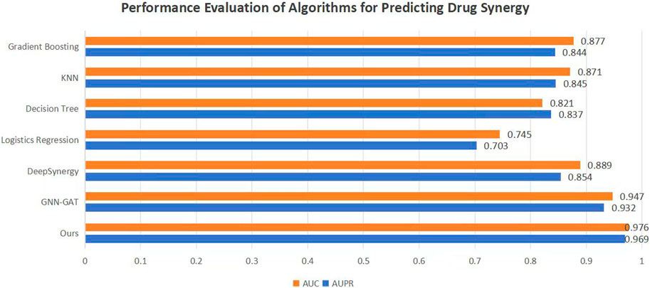
Figure 4. Performance evaluation of algorithms for predicting drug synergy. The bar chart